Glance accepts a model object and returns a tibble::tibble()
with exactly one row of model summaries. The summaries are typically
goodness of fit measures, p-values for hypothesis tests on residuals,
or model convergence information.
Glance never returns information from the original call to the modeling function. This includes the name of the modeling function or any arguments passed to the modeling function.
Glance does not calculate summary measures. Rather, it farms out these
computations to appropriate methods and gathers the results together.
Sometimes a goodness of fit measure will be undefined. In these cases
the measure will be reported as NA.
Glance returns the same number of columns regardless of whether the
model matrix is rank-deficient or not. If so, entries in columns
that no longer have a well-defined value are filled in with an NA
of the appropriate type.
Usage
# S3 method for class 'lmodel2'
glance(x, ...)
Arguments
- x
A
lmodel2object returned bylmodel2::lmodel2().- ...
Additional arguments. Not used. Needed to match generic signature only. Cautionary note: Misspelled arguments will be absorbed in
..., where they will be ignored. If the misspelled argument has a default value, the default value will be used. For example, if you passconf.lvel = 0.9, all computation will proceed usingconf.level = 0.95. Two exceptions here are:
See also
Other lmodel2 tidiers:
tidy.lmodel2()
Value
A tibble::tibble() with exactly one row and columns:
- nobs
Number of observations used.
- p.value
P-value corresponding to the test statistic.
- r.squared
R squared statistic, or the percent of variation explained by the model. Also known as the coefficient of determination.
- theta
Angle between OLS lines `lm(y ~ x)` and `lm(x ~ y)`
- H
H statistic for computing confidence interval of major axis slope
Examples
# load libraries for models and data
library(lmodel2)
data(mod2ex2)
Ex2.res <- lmodel2(Prey ~ Predators, data = mod2ex2, "relative", "relative", 99)
Ex2.res
#>
#> Model II regression
#>
#> Call: lmodel2(formula = Prey ~ Predators, data = mod2ex2,
#> range.y = "relative", range.x = "relative", nperm = 99)
#>
#> n = 20 r = 0.8600787 r-square = 0.7397354
#> Parametric P-values: 2-tailed = 1.161748e-06 1-tailed = 5.808741e-07
#> Angle between the two OLS regression lines = 5.106227 degrees
#>
#> Permutation tests of OLS, MA, RMA slopes: 1-tailed, tail corresponding to sign
#> A permutation test of r is equivalent to a permutation test of the OLS slope
#> P-perm for SMA = NA because the SMA slope cannot be tested
#>
#> Regression results
#> Method Intercept Slope Angle (degrees) P-perm (1-tailed)
#> 1 OLS 20.02675 2.631527 69.19283 0.01
#> 2 MA 13.05968 3.465907 73.90584 0.01
#> 3 SMA 16.45205 3.059635 71.90073 NA
#> 4 RMA 17.25651 2.963292 71.35239 0.01
#>
#> Confidence intervals
#> Method 2.5%-Intercept 97.5%-Intercept 2.5%-Slope 97.5%-Slope
#> 1 OLS 12.490993 27.56251 1.858578 3.404476
#> 2 MA 1.347422 19.76310 2.663101 4.868572
#> 3 SMA 9.195287 22.10353 2.382810 3.928708
#> 4 RMA 8.962997 23.84493 2.174260 3.956527
#>
#> Eigenvalues: 269.8212 6.418234
#>
#> H statistic used for computing C.I. of MA: 0.006120651
#>
# summarize model fit with tidiers + visualization
tidy(Ex2.res)
#> # A tibble: 8 × 6
#> method term estimate conf.low conf.high p.value
#> <chr> <chr> <dbl> <dbl> <dbl> <dbl>
#> 1 MA Intercept 13.1 1.35 19.8 0.01
#> 2 MA Slope 3.47 2.66 4.87 0.01
#> 3 OLS Intercept 20.0 12.5 27.6 0.01
#> 4 OLS Slope 2.63 1.86 3.40 0.01
#> 5 RMA Intercept 17.3 8.96 23.8 0.01
#> 6 RMA Slope 2.96 2.17 3.96 0.01
#> 7 SMA Intercept 16.5 9.20 22.1 NA
#> 8 SMA Slope 3.06 2.38 3.93 NA
glance(Ex2.res)
#> # A tibble: 1 × 5
#> r.squared theta p.value H nobs
#> <dbl> <dbl> <dbl> <dbl> <int>
#> 1 0.740 5.11 0.00000116 0.00612 20
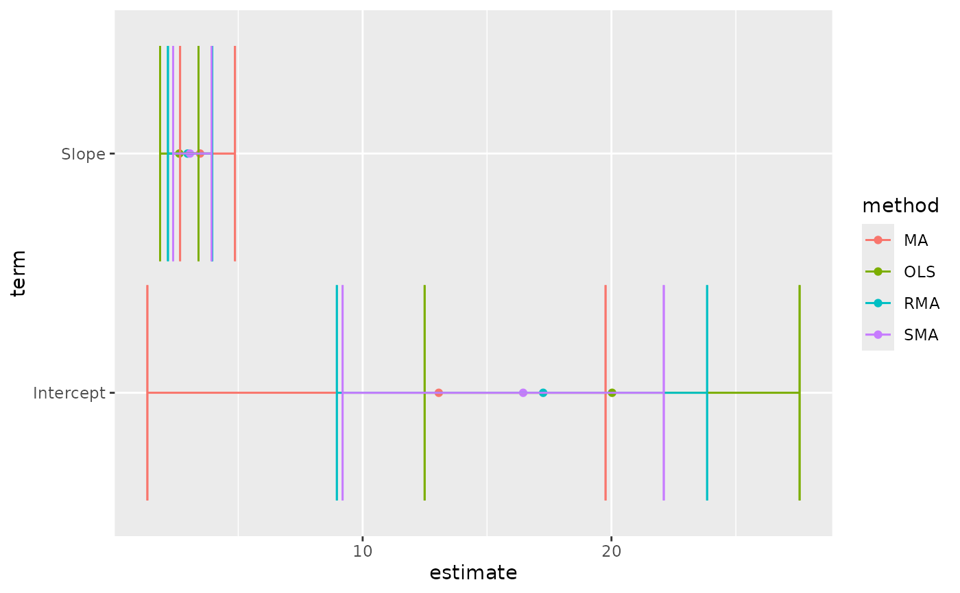
# this allows coefficient plots with ggplot2
library(ggplot2)
ggplot(tidy(Ex2.res), aes(estimate, term, color = method)) +
geom_point() +
geom_errorbarh(aes(xmin = conf.low, xmax = conf.high)) +
geom_errorbarh(aes(xmin = conf.low, xmax = conf.high))