broom and dplyr

2024-09-27

broom and dplyr

While broom is useful for summarizing the result of a single analysis in a consistent format, it is really designed for high-throughput applications, where you must combine results from multiple analyses. These could be subgroups of data, analyses using different models, bootstrap replicates, permutations, and so on. In particular, it plays well with the nest/unnest functions in tidyr and the map function in purrr. First, loading necessary packages and setting some defaults:

library(broom)
library(tibble)
library(ggplot2)
library(dplyr)
library(tidyr)
library(purrr)

theme_set(theme_minimal())

Let’s try this on a simple dataset, the built-in Orange. We start by coercing Orange to a tibble. This gives a nicer print method that will especially useful later on when we start working with list-columns.

data(Orange)

Orange <- as_tibble(Orange)
Orange

## # A tibble: 35 × 3
##    Tree    age circumference
##    <ord> <dbl>         <dbl>
##  1 1       118            30
##  2 1       484            58
##  3 1       664            87
##  4 1      1004           115
##  5 1      1231           120
##  6 1      1372           142
##  7 1      1582           145
##  8 2       118            33
##  9 2       484            69
## 10 2       664           111
## # ℹ 25 more rows

This contains 35 observations of three variables: Tree, age, and circumference. Tree is a factor with five levels describing five trees. As might be expected, age and circumference are correlated:

cor(Orange$age, Orange$circumference)

## [1] 0.9135189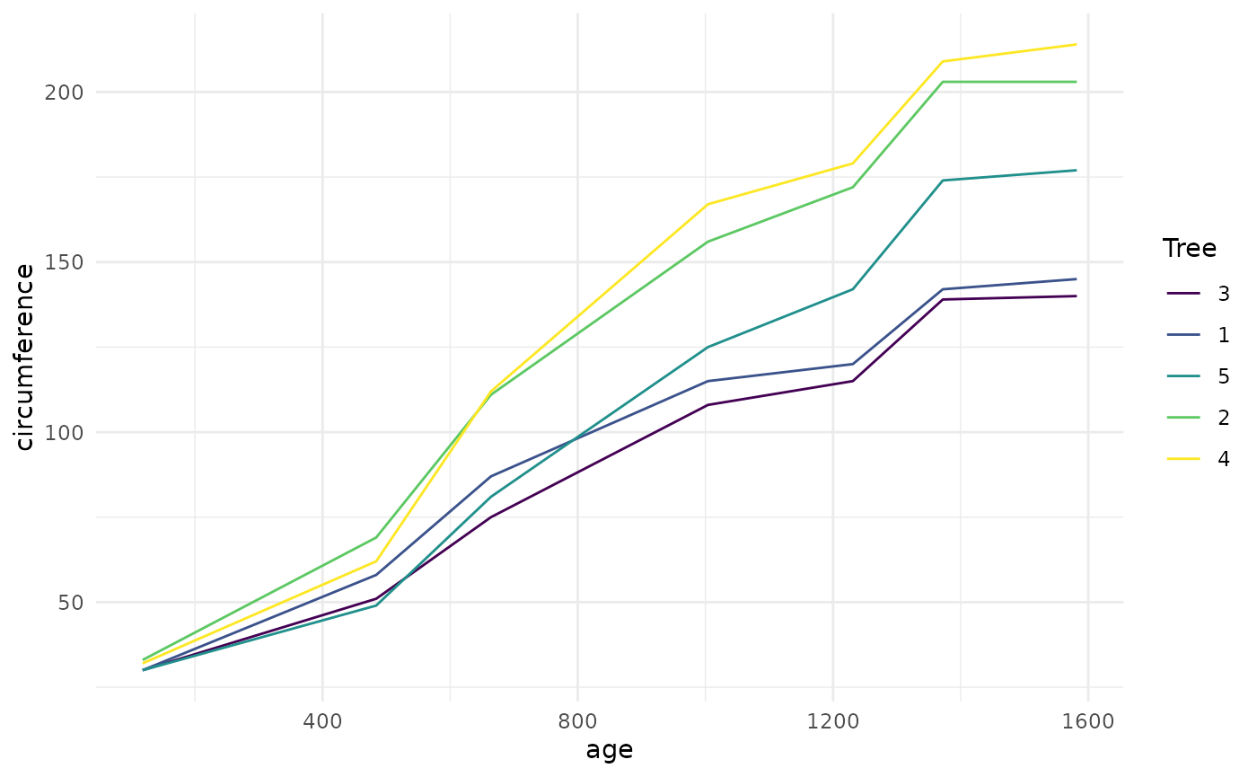

ggplot(Orange, aes(age, circumference, color = Tree)) +
  geom_line()

Suppose you want to test for correlations individually within each tree. You can do this with dplyr’s group_by:

Orange %>%
  group_by(Tree) %>%
  summarize(correlation = cor(age, circumference))

## # A tibble: 5 × 2
##   Tree  correlation
##   <ord>       <dbl>
## 1 3           0.988
## 2 1           0.985
## 3 5           0.988
## 4 2           0.987
## 5 4           0.984

(Note that the correlations are much higher than the aggregated one, and furthermore we can now see it is similar across trees).

Suppose that instead of simply estimating a correlation, we want to perform a hypothesis test with cor.test:

ct <- cor.test(Orange$age, Orange$circumference)
ct

## 
##  Pearson's product-moment correlation
## 
## data:  Orange$age and Orange$circumference
## t = 12.9, df = 33, p-value = 1.931e-14
## alternative hypothesis: true correlation is not equal to 0
## 95 percent confidence interval:
##  0.8342364 0.9557955
## sample estimates:
##       cor 
## 0.9135189

This contains multiple values we could want in our output. Some are vectors of length 1, such as the p-value and the estimate, and some are longer, such as the confidence interval. We can get this into a nicely organized tibble using the tidy function:

tidy(ct)

## # A tibble: 1 × 8
##   estimate statistic  p.value parameter conf.low conf.high method         
##      <dbl>     <dbl>    <dbl>     <int>    <dbl>     <dbl> <chr>          
## 1    0.914      12.9 1.93e-14        33    0.834     0.956 Pearson's prod…
## # ℹ 1 more variable: alternative <chr>

Often, we want to perform multiple tests or fit multiple models, each on a different part of the data. In this case, we recommend a nest-map-unnest workflow. For example, suppose we want to perform correlation tests for each different tree. We start by nesting our data based on the group of interest:

nested <- Orange %>%
  nest(data = -Tree)

Then we run a correlation test for each nested tibble using purrr::map:

nested %>%
  mutate(test = map(data, ~ cor.test(.x$age, .x$circumference)))

## # A tibble: 5 × 3
##   Tree  data             test   
##   <ord> <list>           <list> 
## 1 1     <tibble [7 × 2]> <htest>
## 2 2     <tibble [7 × 2]> <htest>
## 3 3     <tibble [7 × 2]> <htest>
## 4 4     <tibble [7 × 2]> <htest>
## 5 5     <tibble [7 × 2]> <htest>

This results in a list-column of S3 objects. We want to tidy each of the objects, which we can also do with map.

nested %>%
  mutate(
    test = map(data, ~ cor.test(.x$age, .x$circumference)), # S3 list-col
    tidied = map(test, tidy)
  )

## # A tibble: 5 × 4
##   Tree  data             test    tidied          
##   <ord> <list>           <list>  <list>          
## 1 1     <tibble [7 × 2]> <htest> <tibble [1 × 8]>
## 2 2     <tibble [7 × 2]> <htest> <tibble [1 × 8]>
## 3 3     <tibble [7 × 2]> <htest> <tibble [1 × 8]>
## 4 4     <tibble [7 × 2]> <htest> <tibble [1 × 8]>
## 5 5     <tibble [7 × 2]> <htest> <tibble [1 × 8]>

Finally, we want to unnest the tidied data frames so we can see the results in a flat tibble. All together, this looks like:

Orange %>%
  nest(data = -Tree) %>%
  mutate(
    test = map(data, ~ cor.test(.x$age, .x$circumference)), # S3 list-col
    tidied = map(test, tidy)
  ) %>%
  unnest(tidied)

## # A tibble: 5 × 11
##   Tree  data     test    estimate statistic   p.value parameter conf.low
##   <ord> <list>   <list>     <dbl>     <dbl>     <dbl>     <int>    <dbl>
## 1 1     <tibble> <htest>    0.985      13.0 0.0000485         5    0.901
## 2 2     <tibble> <htest>    0.987      13.9 0.0000343         5    0.914
## 3 3     <tibble> <htest>    0.988      14.4 0.0000290         5    0.919
## 4 4     <tibble> <htest>    0.984      12.5 0.0000573         5    0.895
## 5 5     <tibble> <htest>    0.988      14.1 0.0000318         5    0.916
## # ℹ 3 more variables: conf.high <dbl>, method <chr>, alternative <chr>

This workflow becomes even more useful when applied to regressions. Untidy output for a regression looks like:

lm_fit <- lm(age ~ circumference, data = Orange)
summary(lm_fit)

## 
## Call:
## lm(formula = age ~ circumference, data = Orange)
## 
## Residuals:
##     Min      1Q  Median      3Q     Max 
## -317.88 -140.90  -17.20   96.54  471.16 
## 
## Coefficients:
##               Estimate Std. Error t value Pr(>|t|)    
## (Intercept)    16.6036    78.1406   0.212    0.833    
## circumference   7.8160     0.6059  12.900 1.93e-14 ***
## ---
## Signif. codes:  0 '***' 0.001 '**' 0.01 '*' 0.05 '.' 0.1 ' ' 1
## 
## Residual standard error: 203.1 on 33 degrees of freedom
## Multiple R-squared:  0.8345, Adjusted R-squared:  0.8295 
## F-statistic: 166.4 on 1 and 33 DF,  p-value: 1.931e-14

where we tidy these results, we get multiple rows of output for each model:

tidy(lm_fit)

## # A tibble: 2 × 5
##   term          estimate std.error statistic  p.value
##   <chr>            <dbl>     <dbl>     <dbl>    <dbl>
## 1 (Intercept)      16.6     78.1       0.212 8.33e- 1
## 2 circumference     7.82     0.606    12.9   1.93e-14

Now we can handle multiple regressions at once using exactly the same workflow as before:

Orange %>%
  nest(data = -Tree) %>%
  mutate(
    fit = map(data, ~ lm(age ~ circumference, data = .x)),
    tidied = map(fit, tidy)
  ) %>%
  unnest(tidied)

## # A tibble: 10 × 8
##    Tree  data             fit   term  estimate std.error statistic p.value
##    <ord> <list>           <lis> <chr>    <dbl>     <dbl>     <dbl>   <dbl>
##  1 1     <tibble [7 × 2]> <lm>  (Int…  -265.      98.6      -2.68  4.36e-2
##  2 1     <tibble [7 × 2]> <lm>  circ…    11.9      0.919    13.0   4.85e-5
##  3 2     <tibble [7 × 2]> <lm>  (Int…  -132.      83.1      -1.59  1.72e-1
##  4 2     <tibble [7 × 2]> <lm>  circ…     7.80     0.560    13.9   3.43e-5
##  5 3     <tibble [7 × 2]> <lm>  (Int…  -210.      85.3      -2.46  5.74e-2
##  6 3     <tibble [7 × 2]> <lm>  circ…    12.0      0.835    14.4   2.90e-5
##  7 4     <tibble [7 × 2]> <lm>  (Int…   -76.5     88.3      -0.867 4.26e-1
##  8 4     <tibble [7 × 2]> <lm>  circ…     7.17     0.572    12.5   5.73e-5
##  9 5     <tibble [7 × 2]> <lm>  (Int…   -54.5     76.9      -0.709 5.10e-1
## 10 5     <tibble [7 × 2]> <lm>  circ…     8.79     0.621    14.1   3.18e-5

You can just as easily use multiple predictors in the regressions, as shown here on the mtcars dataset. We nest the data into automatic and manual cars (the am column), then perform the regression within each nested tibble.

data(mtcars)
mtcars <- as_tibble(mtcars) # to play nicely with list-cols
mtcars

## # A tibble: 32 × 11
##      mpg   cyl  disp    hp  drat    wt  qsec    vs    am  gear  carb
##    <dbl> <dbl> <dbl> <dbl> <dbl> <dbl> <dbl> <dbl> <dbl> <dbl> <dbl>
##  1  21       6  160    110  3.9   2.62  16.5     0     1     4     4
##  2  21       6  160    110  3.9   2.88  17.0     0     1     4     4
##  3  22.8     4  108     93  3.85  2.32  18.6     1     1     4     1
##  4  21.4     6  258    110  3.08  3.22  19.4     1     0     3     1
##  5  18.7     8  360    175  3.15  3.44  17.0     0     0     3     2
##  6  18.1     6  225    105  2.76  3.46  20.2     1     0     3     1
##  7  14.3     8  360    245  3.21  3.57  15.8     0     0     3     4
##  8  24.4     4  147.    62  3.69  3.19  20       1     0     4     2
##  9  22.8     4  141.    95  3.92  3.15  22.9     1     0     4     2
## 10  19.2     6  168.   123  3.92  3.44  18.3     1     0     4     4
## # ℹ 22 more rows

mtcars %>%
  nest(data = -am) %>%
  mutate(
    fit = map(data, ~ lm(wt ~ mpg + qsec + gear, data = .x)), # S3 list-col
    tidied = map(fit, tidy)
  ) %>%
  unnest(tidied)

## # A tibble: 8 × 8
##      am data     fit    term        estimate std.error statistic  p.value
##   <dbl> <list>   <list> <chr>          <dbl>     <dbl>     <dbl>    <dbl>
## 1     1 <tibble> <lm>   (Intercept)   4.28      3.46      1.24   0.247   
## 2     1 <tibble> <lm>   mpg          -0.101     0.0294   -3.43   0.00750 
## 3     1 <tibble> <lm>   qsec          0.0398    0.151     0.264  0.798   
## 4     1 <tibble> <lm>   gear         -0.0229    0.349    -0.0656 0.949   
## 5     0 <tibble> <lm>   (Intercept)   4.92      1.40      3.52   0.00309 
## 6     0 <tibble> <lm>   mpg          -0.192     0.0443   -4.33   0.000591
## 7     0 <tibble> <lm>   qsec          0.0919    0.0983    0.935  0.365   
## 8     0 <tibble> <lm>   gear          0.147     0.368     0.398  0.696

What if you want not just the tidy output, but the augment and glance outputs as well, while still performing each regression only once? Since we’re using list-columns, we can just fit the model once and use multiple list-columns to store the tidied, glanced and augmented outputs.

regressions <- mtcars %>%
  nest(data = -am) %>%
  mutate(
    fit = map(data, ~ lm(wt ~ mpg + qsec + gear, data = .x)),
    tidied = map(fit, tidy),
    glanced = map(fit, glance),
    augmented = map(fit, augment)
  )

regressions %>%
  unnest(tidied)

## # A tibble: 8 × 10
##      am data     fit   term  estimate std.error statistic p.value glanced 
##   <dbl> <list>   <lis> <chr>    <dbl>     <dbl>     <dbl>   <dbl> <list>  
## 1     1 <tibble> <lm>  (Int…   4.28      3.46      1.24   2.47e-1 <tibble>
## 2     1 <tibble> <lm>  mpg    -0.101     0.0294   -3.43   7.50e-3 <tibble>
## 3     1 <tibble> <lm>  qsec    0.0398    0.151     0.264  7.98e-1 <tibble>
## 4     1 <tibble> <lm>  gear   -0.0229    0.349    -0.0656 9.49e-1 <tibble>
## 5     0 <tibble> <lm>  (Int…   4.92      1.40      3.52   3.09e-3 <tibble>
## 6     0 <tibble> <lm>  mpg    -0.192     0.0443   -4.33   5.91e-4 <tibble>
## 7     0 <tibble> <lm>  qsec    0.0919    0.0983    0.935  3.65e-1 <tibble>
## 8     0 <tibble> <lm>  gear    0.147     0.368     0.398  6.96e-1 <tibble>
## # ℹ 1 more variable: augmented <list>

regressions %>%
  unnest(glanced)

## # A tibble: 2 × 17
##      am data     fit    tidied   r.squared adj.r.squared sigma statistic
##   <dbl> <list>   <list> <list>       <dbl>         <dbl> <dbl>     <dbl>
## 1     1 <tibble> <lm>   <tibble>     0.833         0.778 0.291     15.0 
## 2     0 <tibble> <lm>   <tibble>     0.625         0.550 0.522      8.32
## # ℹ 9 more variables: p.value <dbl>, df <dbl>, logLik <dbl>, AIC <dbl>,
## #   BIC <dbl>, deviance <dbl>, df.residual <int>, nobs <int>,
## #   augmented <list>

regressions %>%
  unnest(augmented)

## # A tibble: 32 × 15
##       am data     fit    tidied   glanced     wt   mpg  qsec  gear .fitted
##    <dbl> <list>   <list> <list>   <list>   <dbl> <dbl> <dbl> <dbl>   <dbl>
##  1     1 <tibble> <lm>   <tibble> <tibble>  2.62  21    16.5     4    2.73
##  2     1 <tibble> <lm>   <tibble> <tibble>  2.88  21    17.0     4    2.75
##  3     1 <tibble> <lm>   <tibble> <tibble>  2.32  22.8  18.6     4    2.63
##  4     1 <tibble> <lm>   <tibble> <tibble>  2.2   32.4  19.5     4    1.70
##  5     1 <tibble> <lm>   <tibble> <tibble>  1.62  30.4  18.5     4    1.86
##  6     1 <tibble> <lm>   <tibble> <tibble>  1.84  33.9  19.9     4    1.56
##  7     1 <tibble> <lm>   <tibble> <tibble>  1.94  27.3  18.9     4    2.19
##  8     1 <tibble> <lm>   <tibble> <tibble>  2.14  26    16.7     5    2.21
##  9     1 <tibble> <lm>   <tibble> <tibble>  1.51  30.4  16.9     5    1.77
## 10     1 <tibble> <lm>   <tibble> <tibble>  3.17  15.8  14.5     5    3.15
## # ℹ 22 more rows
## # ℹ 5 more variables: .resid <dbl>, .hat <dbl>, .sigma <dbl>,
## #   .cooksd <dbl>, .std.resid <dbl>

By combining the estimates and p-values across all groups into the same tidy data frame (instead of a list of output model objects), a new class of analyses and visualizations becomes straightforward. This includes

• Sorting by p-value or estimate to find the most significant terms across all tests
• P-value histograms
• Volcano plots comparing p-values to effect size estimates

In each of these cases, we can easily filter, facet, or distinguish based on the term column. In short, this makes the tools of tidy data analysis available for the results of data analysis and models, not just the inputs.