Tidy summarizes information about the components of a model. A model component might be a single term in a regression, a single hypothesis, a cluster, or a class. Exactly what tidy considers to be a model component varies across models but is usually self-evident. If a model has several distinct types of components, you will need to specify which components to return.
Usage
# S3 method for class 'kappa'
tidy(x, ...)
Arguments
- x
A
kappaobject returned frompsych::cohen.kappa().- ...
Additional arguments. Not used. Needed to match generic signature only. Cautionary note: Misspelled arguments will be absorbed in
..., where they will be ignored. If the misspelled argument has a default value, the default value will be used. For example, if you passconf.lvel = 0.9, all computation will proceed usingconf.level = 0.95. Two exceptions here are:
Details
Note that confidence level (alpha) for the confidence interval
cannot be set in tidy. Instead you must set the alpha argument
to psych::cohen.kappa() when creating the kappa object.
Value
A tibble::tibble() with columns:
- conf.high
Upper bound on the confidence interval for the estimate.
- conf.low
Lower bound on the confidence interval for the estimate.
- estimate
The estimated value of the regression term.
- type
Either `weighted` or `unweighted`.
Examples
# load libraries for models and data
library(psych)
#>
#> Attaching package: ‘psych’
#> The following object is masked from ‘package:boot’:
#>
#> logit
#> The following object is masked from ‘package:lavaan’:
#>
#> cor2cov
#> The following object is masked from ‘package:car’:
#>
#> logit
#> The following object is masked from ‘package:drc’:
#>
#> logistic
#> The following objects are masked from ‘package:ggplot2’:
#>
#> %+%, alpha
#> The following object is masked from ‘package:mclust’:
#>
#> sim
# generate example data
rater1 <- 1:9
rater2 <- c(1, 3, 1, 6, 1, 5, 5, 6, 7)
# fit model
ck <- cohen.kappa(cbind(rater1, rater2))
# summarize model fit with tidiers + visualization
tidy(ck)
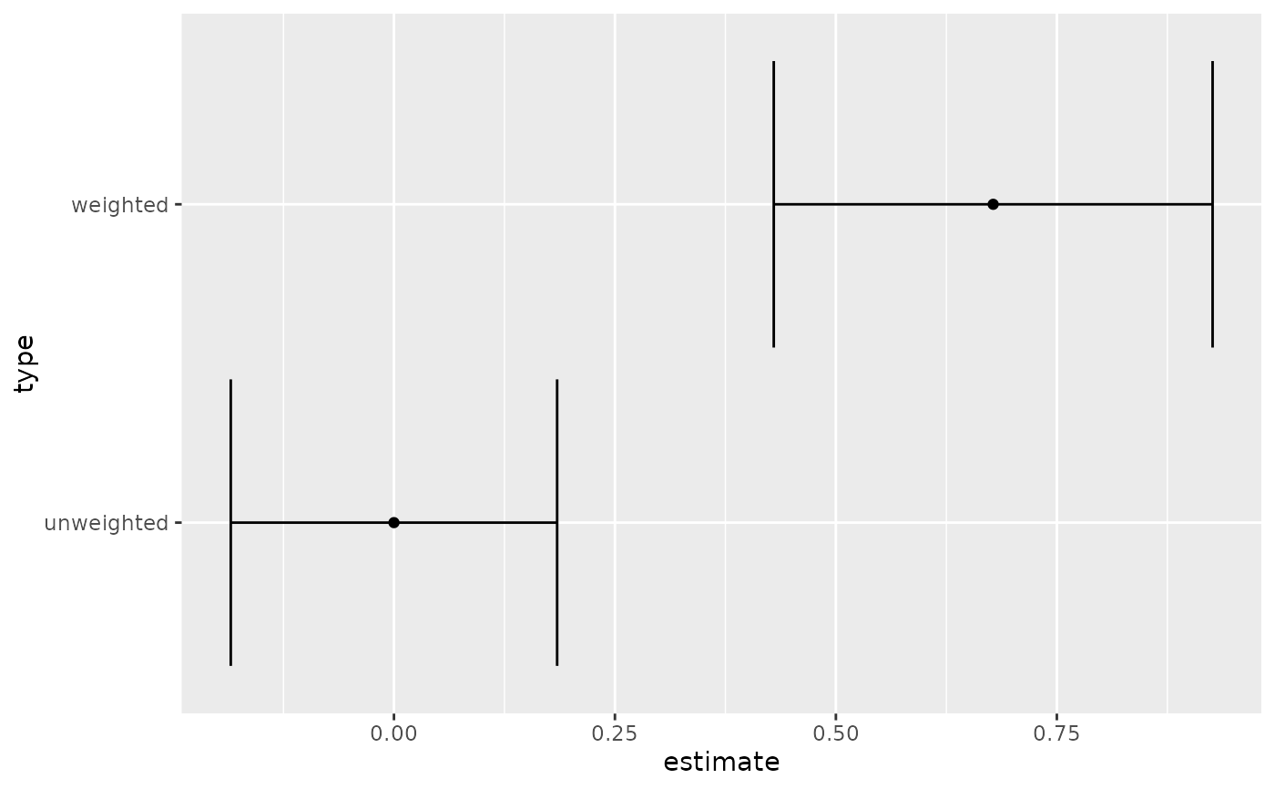
#> # A tibble: 2 × 4
#> type estimate conf.low conf.high
#> <chr> <dbl> <dbl> <dbl>
#> 1 unweighted 0 -0.185 0.185
#> 2 weighted 0.678 0.430 0.926
# graph the confidence intervals
library(ggplot2)
ggplot(tidy(ck), aes(estimate, type)) +
geom_point() +
geom_errorbarh(aes(xmin = conf.low, xmax = conf.high))