Tidy a(n) map object

Tidy summarizes information about the components of a model. A model component might be a single term in a regression, a single hypothesis, a cluster, or a class. Exactly what tidy considers to be a model component varies across models but is usually self-evident. If a model has several distinct types of components, you will need to specify which components to return.

Usage

# S3 method for map
tidy(x, ...)

Arguments

x

A map object returned from maps::map().

...

Additional arguments. Not used. Needed to match generic signature only. Cautionary note: Misspelled arguments will be absorbed in ..., where they will be ignored. If the misspelled argument has a default value, the default value will be used. For example, if you pass conf.lvel = 0.9, all computation will proceed using conf.level = 0.95. Two exceptions here are:

• tidy() methods will warn when supplied an exponentiate argument if it will be ignored.

• augment() methods will warn when supplied a newdata argument if it will be ignored.

See also

tidy(), maps::map()

Value

A tibble::tibble() with columns:

term

The name of the regression term.

long

Longitude.

lat

Latitude.

Remaining columns give information on geographic attributes and depend on the inputted map object. See ?maps::map for more information.

Examples

# load libraries for models and data
library(maps)
#> 
#> Attaching package: ‘maps’
#> The following object is masked from ‘package:cluster’:
#> 
#>     votes.repub
#> The following object is masked from ‘package:purrr’:
#> 
#>     map
#> The following object is masked from ‘package:mclust’:
#> 
#>     map
library(ggplot2)

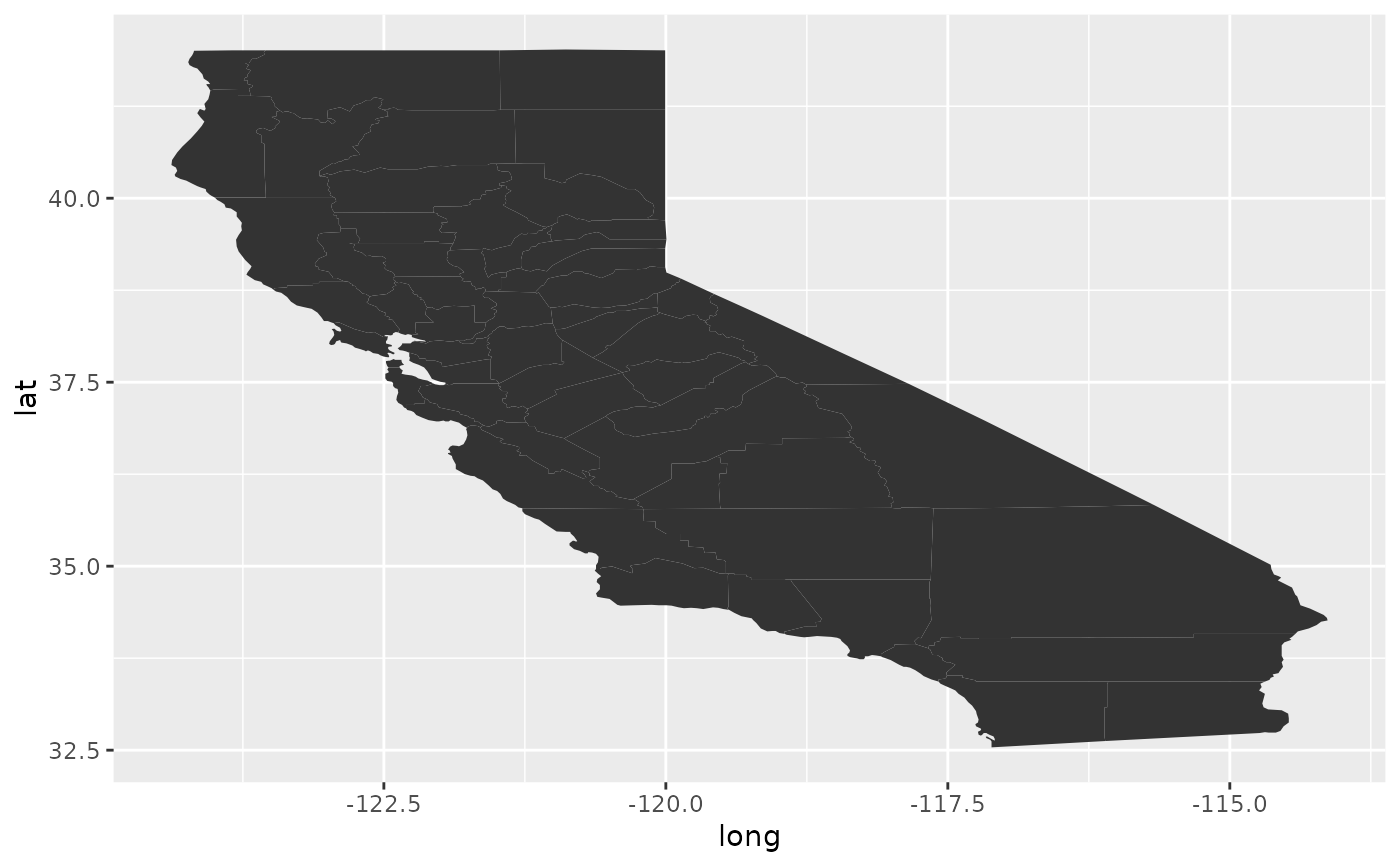
ca <- map("county", "ca", plot = FALSE, fill = TRUE)

tidy(ca)
#> # A tibble: 2,977 × 7
#>    term   long   lat group order region     subregion
#>    <chr> <dbl> <dbl> <dbl> <int> <chr>      <chr>    
#>  1 1     -121.  37.5     1     1 california alameda  
#>  2 2     -122.  37.5     1     2 california alameda  
#>  3 3     -122.  37.5     1     3 california alameda  
#>  4 4     -122.  37.5     1     4 california alameda  
#>  5 5     -122.  37.5     1     5 california alameda  
#>  6 6     -122.  37.5     1     6 california alameda  
#>  7 7     -122.  37.5     1     7 california alameda  
#>  8 8     -122.  37.5     1     8 california alameda  
#>  9 9     -122.  37.5     1     9 california alameda  
#> 10 10    -122.  37.5     1    10 california alameda  
#> # ℹ 2,967 more rows

qplot(long, lat, data = ca, geom = "polygon", group = group)
#> Warning: `qplot()` was deprecated in ggplot2 3.4.0.


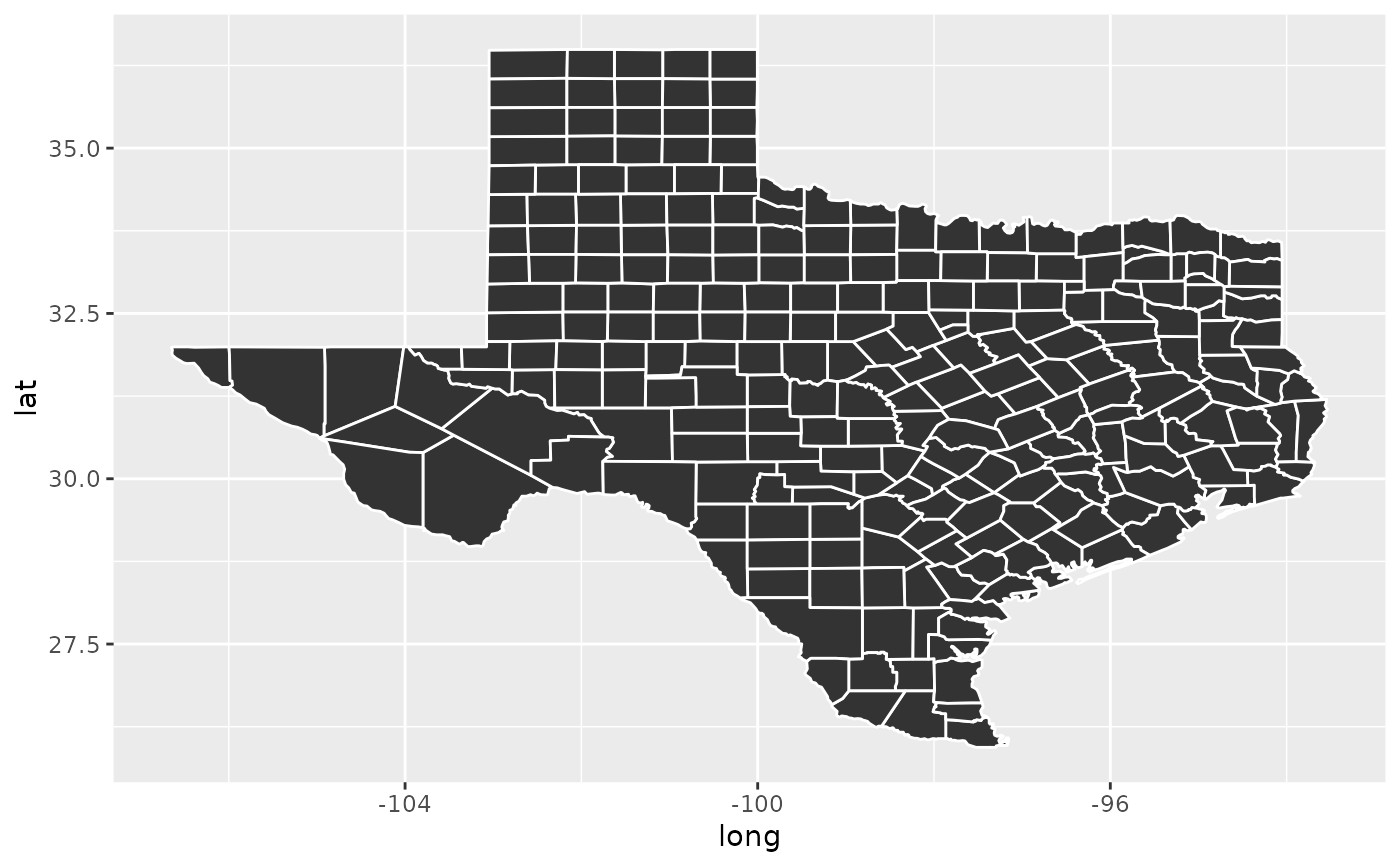
tx <- map("county", "texas", plot = FALSE, fill = TRUE)
tidy(tx)
#> # A tibble: 4,488 × 7
#>    term   long   lat group order region subregion
#>    <chr> <dbl> <dbl> <dbl> <int> <chr>  <chr>    
#>  1 1     -95.8  31.5     1     1 texas  anderson 
#>  2 2     -95.8  31.6     1     2 texas  anderson 
#>  3 3     -95.8  31.6     1     3 texas  anderson 
#>  4 4     -95.7  31.6     1     4 texas  anderson 
#>  5 5     -95.7  31.6     1     5 texas  anderson 
#>  6 6     -95.7  31.6     1     6 texas  anderson 
#>  7 7     -95.8  31.7     1     7 texas  anderson 
#>  8 8     -95.8  31.7     1     8 texas  anderson 
#>  9 9     -95.8  31.6     1     9 texas  anderson 
#> 10 10    -95.8  31.6     1    10 texas  anderson 
#> # ℹ 4,478 more rows
qplot(long, lat,
  data = tx, geom = "polygon", group = group,
  colour = I("white")
)