Tidy a(n) prcomp object

Tidy summarizes information about the components of a model. A model component might be a single term in a regression, a single hypothesis, a cluster, or a class. Exactly what tidy considers to be a model component varies across models but is usually self-evident. If a model has several distinct types of components, you will need to specify which components to return.

Usage

# S3 method for prcomp
tidy(x, matrix = "u", ...)

Arguments

x

A prcomp object returned by stats::prcomp().

matrix

Character specifying which component of the PCA should be tidied.

"u", "samples", "scores", or "x": returns information about the map from the original space into principle components space.
"v", "rotation", "loadings" or "variables": returns information about the map from principle components space back into the original space.
"d", "eigenvalues" or "pcs": returns information about the eigenvalues.

...

Additional arguments. Not used. Needed to match generic signature only. Cautionary note: Misspelled arguments will be absorbed in ..., where they will be ignored. If the misspelled argument has a default value, the default value will be used. For example, if you pass conf.lvel = 0.9, all computation will proceed using conf.level = 0.95. Two exceptions here are:

tidy() methods will warn when supplied an exponentiate argument if it will be ignored.
augment() methods will warn when supplied a newdata argument if it will be ignored.

Value

A tibble::tibble with columns depending on the component of PCA being tidied.

If matrix is "u", "samples", "scores", or "x" each row in the tidied output corresponds to the original data in PCA space. The columns are:

row: ID of the original observation (i.e. rowname from original data).
PC: Integer indicating a principal component.
value: The score of the observation for that particular principal component. That is, the location of the observation in PCA space.

If matrix is "v", "rotation", "loadings" or "variables", each row in the tidied output corresponds to information about the principle components in the original space. The columns are:

row: The variable labels (colnames) of the data set on which PCA was performed.
PC: An integer vector indicating the principal component.
value: The value of the eigenvector (axis score) on the indicated principal component.

If matrix is "d", "eigenvalues" or "pcs", the columns are:

PC: An integer vector indicating the principal component.
std.dev: Standard deviation explained by this PC.
percent: Fraction of variation explained by this component (a numeric value between 0 and 1).
cumulative: Cumulative fraction of variation explained by principle components up to this component (a numeric value between 0 and 1).

Details

See https://stats.stackexchange.com/questions/134282/relationship-between-svd-and-pca-how-to-use-svd-to-perform-pca for information on how to interpret the various tidied matrices. Note that SVD is only equivalent to PCA on centered data.

Examples


pc <- prcomp(USArrests, scale = TRUE)

# information about rotation
tidy(pc)
#> # A tibble: 200 × 3
#>    row        PC  value
#>    <chr>   <dbl>  <dbl>
#>  1 Alabama     1 -0.976
#>  2 Alabama     2 -1.12 
#>  3 Alabama     3  0.440
#>  4 Alabama     4  0.155
#>  5 Alaska      1 -1.93 
#>  6 Alaska      2 -1.06 
#>  7 Alaska      3 -2.02 
#>  8 Alaska      4 -0.434
#>  9 Arizona     1 -1.75 
#> 10 Arizona     2  0.738
#> # ℹ 190 more rows

# information about samples (states)
tidy(pc, "samples")
#> # A tibble: 200 × 3
#>    row        PC  value
#>    <chr>   <dbl>  <dbl>
#>  1 Alabama     1 -0.976
#>  2 Alabama     2 -1.12 
#>  3 Alabama     3  0.440
#>  4 Alabama     4  0.155
#>  5 Alaska      1 -1.93 
#>  6 Alaska      2 -1.06 
#>  7 Alaska      3 -2.02 
#>  8 Alaska      4 -0.434
#>  9 Arizona     1 -1.75 
#> 10 Arizona     2  0.738
#> # ℹ 190 more rows

# information about PCs
tidy(pc, "pcs")
#> # A tibble: 4 × 4
#>      PC std.dev percent cumulative
#>   <dbl>   <dbl>   <dbl>      <dbl>
#> 1     1   1.57   0.620       0.620
#> 2     2   0.995  0.247       0.868
#> 3     3   0.597  0.0891      0.957
#> 4     4   0.416  0.0434      1    

# state map
library(dplyr)
library(ggplot2)
library(maps)

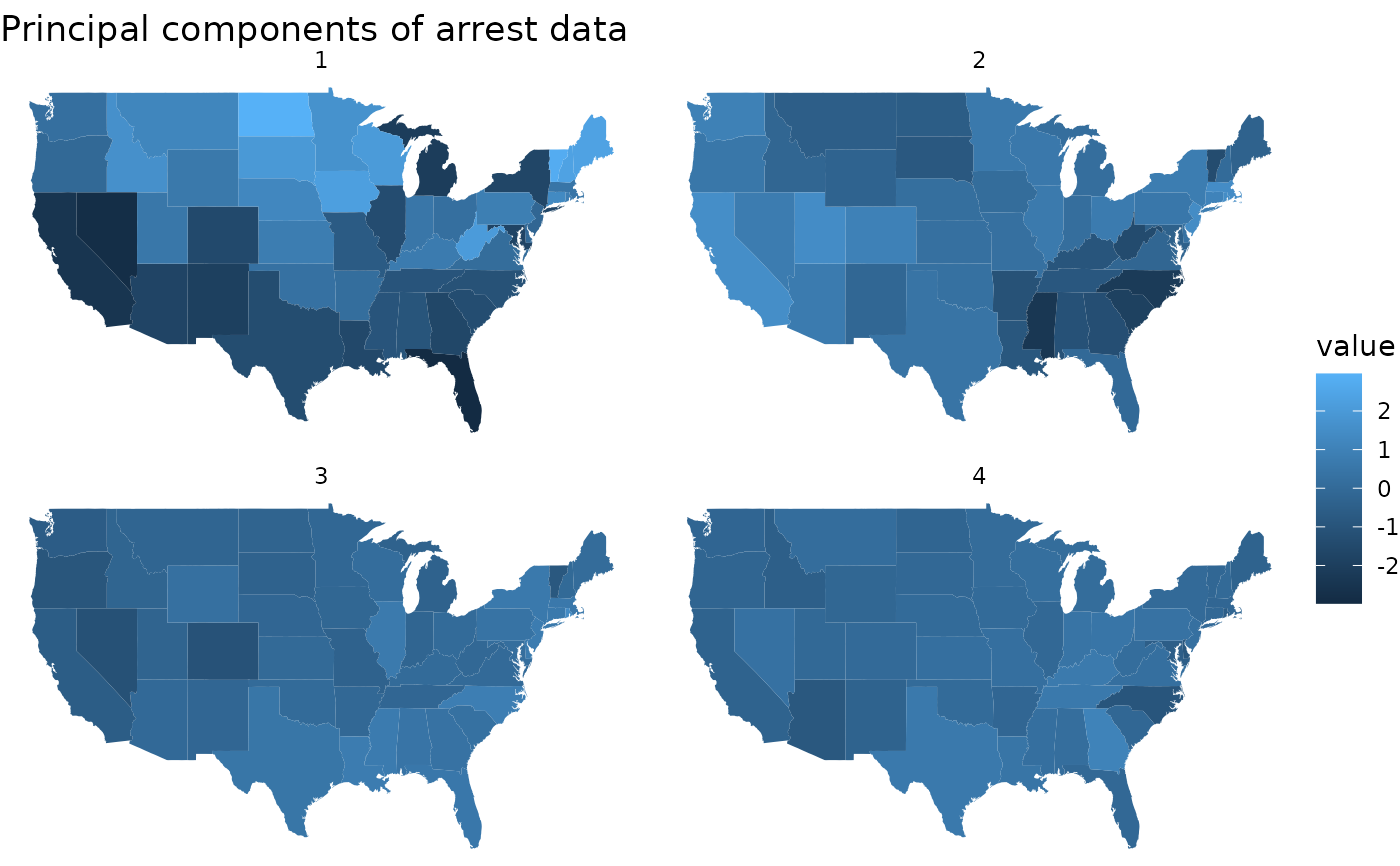
pc %>%
  tidy(matrix = "samples") %>%
  mutate(region = tolower(row)) %>%
  inner_join(map_data("state"), by = "region") %>%
  ggplot(aes(long, lat, group = group, fill = value)) +
  geom_polygon() +
  facet_wrap(~PC) +
  theme_void() +
  ggtitle("Principal components of arrest data")
#> Warning: Detected an unexpected many-to-many relationship between `x` and `y`.
#> ℹ Row 1 of `x` matches multiple rows in `y`.
#> ℹ Row 1 of `y` matches multiple rows in `x`.
#> ℹ If a many-to-many relationship is expected, set `relationship =
#>   "many-to-many"` to silence this warning.


au <- augment(pc, data = USArrests)

au
#> # A tibble: 50 × 9
#>    .rownames   Murder Assault UrbanPop  Rape .fittedPC1 .fittedPC2
#>    <chr>        <dbl>   <int>    <int> <dbl>      <dbl>      <dbl>
#>  1 Alabama       13.2     236       58  21.2    -0.976     -1.12  
#>  2 Alaska        10       263       48  44.5    -1.93      -1.06  
#>  3 Arizona        8.1     294       80  31      -1.75       0.738 
#>  4 Arkansas       8.8     190       50  19.5     0.140     -1.11  
#>  5 California     9       276       91  40.6    -2.50       1.53  
#>  6 Colorado       7.9     204       78  38.7    -1.50       0.978 
#>  7 Connecticut    3.3     110       77  11.1     1.34       1.08  
#>  8 Delaware       5.9     238       72  15.8    -0.0472     0.322 
#>  9 Florida       15.4     335       80  31.9    -2.98      -0.0388
#> 10 Georgia       17.4     211       60  25.8    -1.62      -1.27  
#> # ℹ 40 more rows
#> # ℹ 2 more variables: .fittedPC3 <dbl>, .fittedPC4 <dbl>

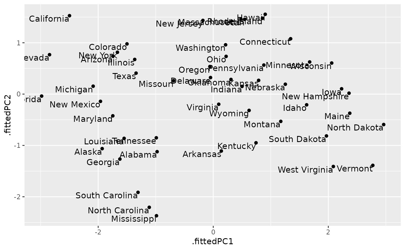
ggplot(au, aes(.fittedPC1, .fittedPC2)) +
  geom_point() +
  geom_text(aes(label = .rownames), vjust = 1, hjust = 1)

Usage

Arguments

Value

Details

See also

Examples