Tidy summarizes information about the components of a model. A model component might be a single term in a regression, a single hypothesis, a cluster, or a class. Exactly what tidy considers to be a model component varies across models but is usually self-evident. If a model has several distinct types of components, you will need to specify which components to return.
Usage
# S3 method for class 'roc'
tidy(x, ...)
Arguments
- x
An
rocobject returned from a call toAUC::roc().- ...
Additional arguments. Not used. Needed to match generic signature only. Cautionary note: Misspelled arguments will be absorbed in
..., where they will be ignored. If the misspelled argument has a default value, the default value will be used. For example, if you passconf.lvel = 0.9, all computation will proceed usingconf.level = 0.95. Two exceptions here are:
Value
A tibble::tibble() with columns:
- cutoff
The cutoff used for classification. Observations with predicted probabilities above this value were assigned class 1, and observations with predicted probabilities below this value were assigned class 0.
- fpr
False positive rate.
- tpr
The true positive rate at the given cutoff.
Examples
# load libraries for models and data
library(AUC)
#> AUC 0.3.2
#> Type AUCNews() to see the change log and ?AUC to get an overview.
#>
#> Attaching package: ‘AUC’
#> The following objects are masked from ‘package:caret’:
#>
#> sensitivity, specificity
# load data
data(churn)
# fit model
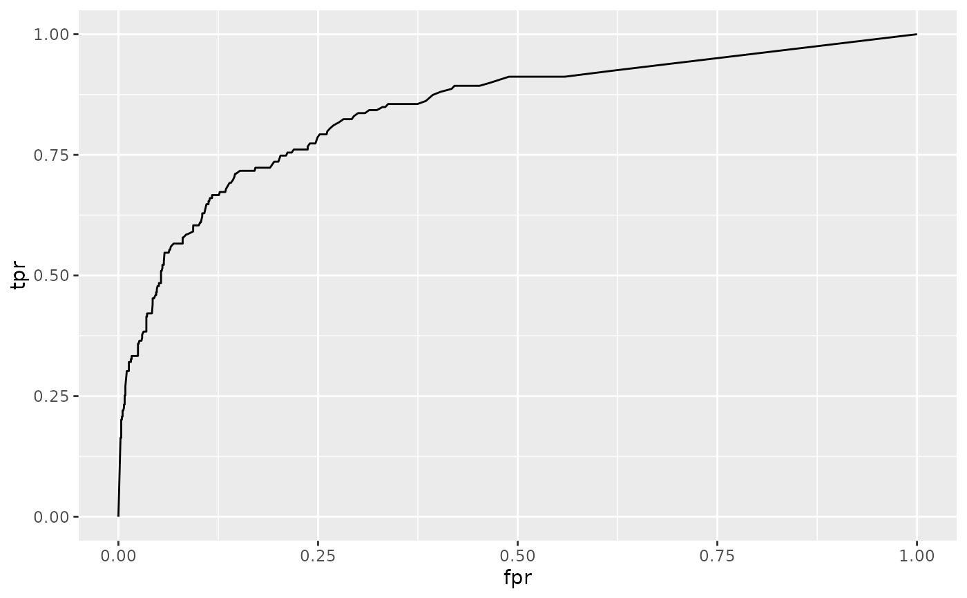
r <- roc(churn$predictions, churn$labels)
# summarize with tidiers + visualization
td <- tidy(r)
td
#> # A tibble: 220 × 3
#> cutoff fpr tpr
#> <dbl> <dbl> <dbl>
#> 1 1 0 0
#> 2 1 0.00262 0.164
#> 3 0.972 0.00350 0.164
#> 4 0.968 0.00350 0.182
#> 5 0.964 0.00350 0.189
#> 6 0.96 0.00350 0.201
#> 7 0.932 0.00437 0.201
#> 8 0.91 0.00437 0.208
#> 9 0.908 0.00525 0.208
#> 10 0.902 0.00525 0.214
#> # ℹ 210 more rows
library(ggplot2)
ggplot(td, aes(fpr, tpr)) +
geom_line()
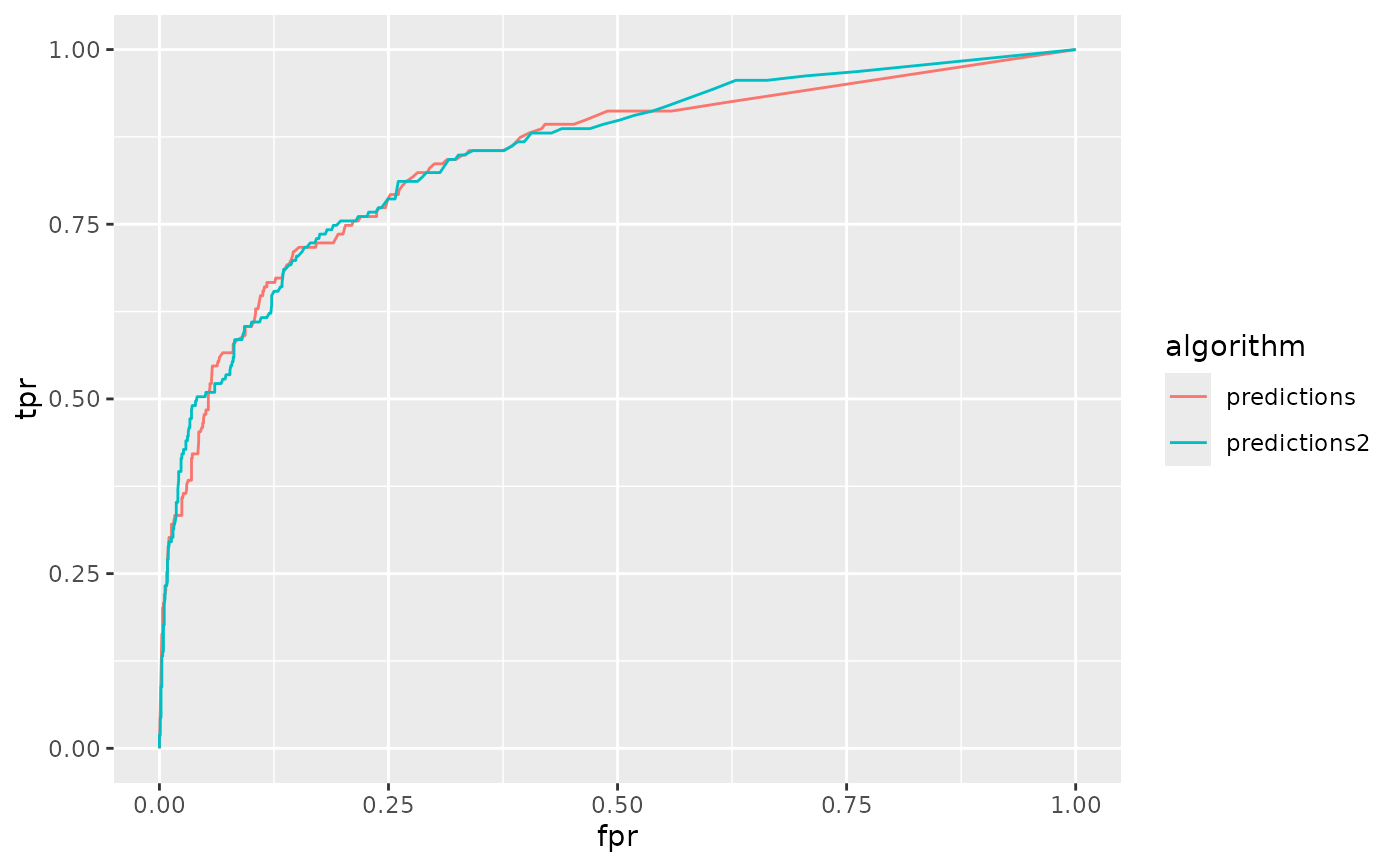
 # compare the ROC curves for two prediction algorithms
library(dplyr)
library(tidyr)
rocs <- churn |>
pivot_longer(contains("predictions"),
names_to = "algorithm",
values_to = "value"
) |>
nest(data = -algorithm) |>
mutate(tidy_roc = purrr::map(data, \(x) tidy(roc(x$value, x$labels)))) |>
unnest(tidy_roc)
ggplot(rocs, aes(fpr, tpr, color = algorithm)) +
geom_line()
# compare the ROC curves for two prediction algorithms
library(dplyr)
library(tidyr)
rocs <- churn |>
pivot_longer(contains("predictions"),
names_to = "algorithm",
values_to = "value"
) |>
nest(data = -algorithm) |>
mutate(tidy_roc = purrr::map(data, \(x) tidy(roc(x$value, x$labels)))) |>
unnest(tidy_roc)
ggplot(rocs, aes(fpr, tpr, color = algorithm)) +
geom_line()