Augment data with information from a(n) nls object

Augment accepts a model object and a dataset and adds information about each observation in the dataset. Most commonly, this includes predicted values in the .fitted column, residuals in the .resid column, and standard errors for the fitted values in a .se.fit column. New columns always begin with a . prefix to avoid overwriting columns in the original dataset.

Users may pass data to augment via either the data argument or the newdata argument. If the user passes data to the data argument, it must be exactly the data that was used to fit the model object. Pass datasets to newdata to augment data that was not used during model fitting. This still requires that at least all predictor variable columns used to fit the model are present. If the original outcome variable used to fit the model is not included in newdata, then no .resid column will be included in the output.

Augment will often behave differently depending on whether data or newdata is given. This is because there is often information associated with training observations (such as influences or related) measures that is not meaningfully defined for new observations.

For convenience, many augment methods provide default data arguments, so that augment(fit) will return the augmented training data. In these cases, augment tries to reconstruct the original data based on the model object with varying degrees of success.

The augmented dataset is always returned as a tibble::tibble with the same number of rows as the passed dataset. This means that the passed data must be coercible to a tibble. If a predictor enters the model as part of a matrix of covariates, such as when the model formula uses splines::ns(), stats::poly(), or survival::Surv(), it is represented as a matrix column.

We are in the process of defining behaviors for models fit with various na.action arguments, but make no guarantees about behavior when data is missing at this time.

Usage

# S3 method for nls
augment(x, data = NULL, newdata = NULL, ...)

Arguments

x

An nls object returned from stats::nls().

data

A base::data.frame or tibble::tibble() containing the original data that was used to produce the object x. Defaults to stats::model.frame(x) so that augment(my_fit) returns the augmented original data. Do not pass new data to the data argument. Augment will report information such as influence and cooks distance for data passed to the data argument. These measures are only defined for the original training data.

newdata

A base::data.frame() or tibble::tibble() containing all the original predictors used to create x. Defaults to NULL, indicating that nothing has been passed to newdata. If newdata is specified, the data argument will be ignored.

...

Additional arguments. Not used. Needed to match generic signature only. Cautionary note: Misspelled arguments will be absorbed in ..., where they will be ignored. If the misspelled argument has a default value, the default value will be used. For example, if you pass conf.lvel = 0.9, all computation will proceed using conf.level = 0.95. Two exceptions here are:

tidy() methods will warn when supplied an exponentiate argument if it will be ignored.
augment() methods will warn when supplied a newdata argument if it will be ignored.

Details

augment.nls does not currently support confidence intervals due to a lack of support in stats::predict.nls().

Value

A tibble::tibble() with columns:

.fitted: Fitted or predicted value.
.resid: The difference between observed and fitted values.

Examples


# fit model
n <- nls(mpg ~ k * e^wt, data = mtcars, start = list(k = 1, e = 2))

# summarize model fit with tidiers + visualization
tidy(n)
#> # A tibble: 2 × 5
#>   term  estimate std.error statistic  p.value
#>   <chr>    <dbl>     <dbl>     <dbl>    <dbl>
#> 1 k       49.7      3.79        13.1 5.96e-14
#> 2 e        0.746    0.0199      37.5 8.86e-27
augment(n)
#> # A tibble: 32 × 4
#>      mpg    wt .fitted .resid
#>    <dbl> <dbl>   <dbl>  <dbl>
#>  1  21    2.62    23.0 -2.01 
#>  2  21    2.88    21.4 -0.352
#>  3  22.8  2.32    25.1 -2.33 
#>  4  21.4  3.22    19.3  2.08 
#>  5  18.7  3.44    18.1  0.611
#>  6  18.1  3.46    18.0  0.117
#>  7  14.3  3.57    17.4 -3.11 
#>  8  24.4  3.19    19.5  4.93 
#>  9  22.8  3.15    19.7  3.10 
#> 10  19.2  3.44    18.1  1.11 
#> # ℹ 22 more rows
glance(n)
#> # A tibble: 1 × 9
#>   sigma isConv     finTol logLik   AIC   BIC deviance df.residual  nobs
#>   <dbl> <lgl>       <dbl>  <dbl> <dbl> <dbl>    <dbl>       <int> <int>
#> 1  2.67 TRUE   0.00000204  -75.8  158.  162.     214.          30    32

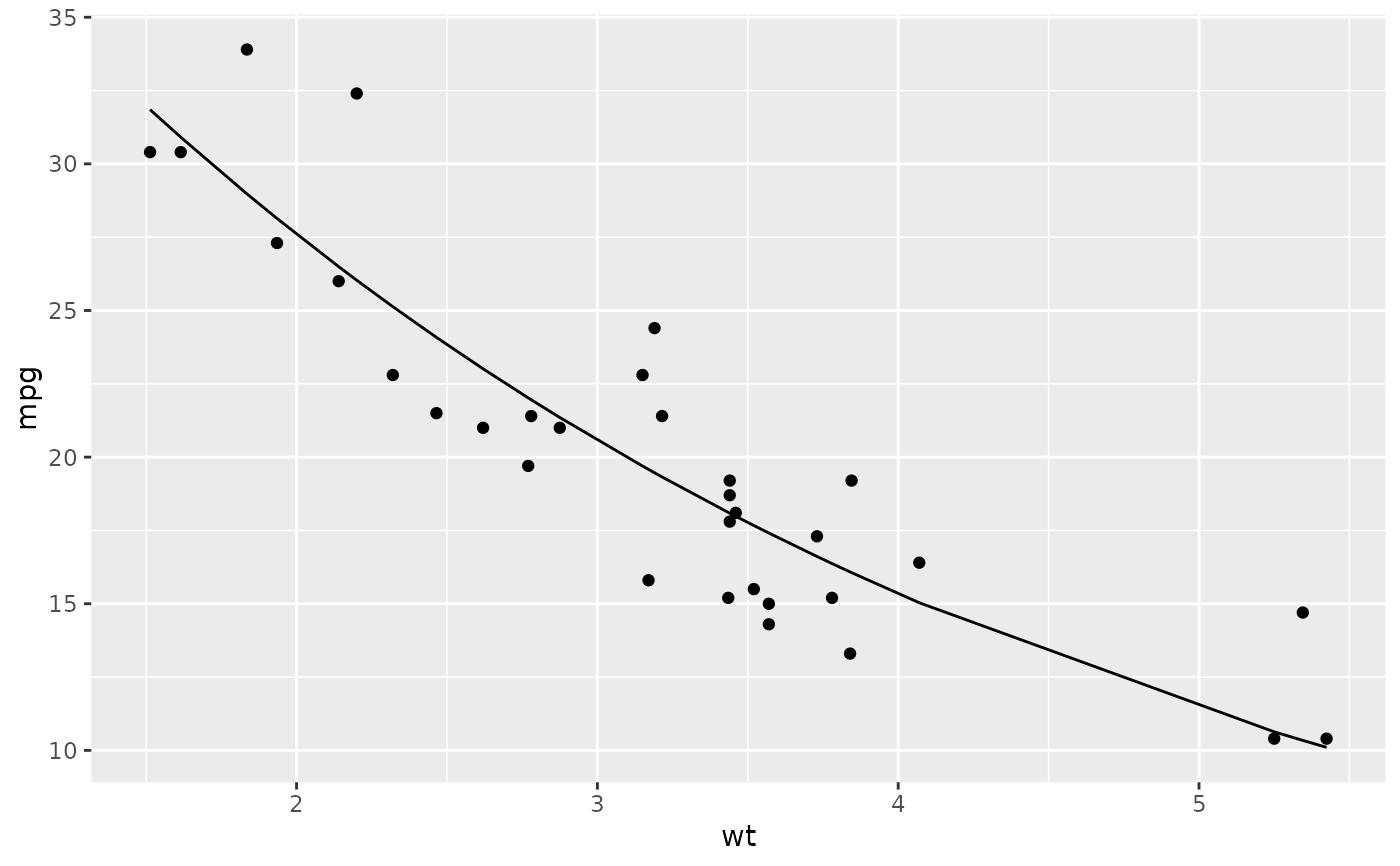
library(ggplot2)

ggplot(augment(n), aes(wt, mpg)) +
  geom_point() +
  geom_line(aes(y = .fitted))


newdata <- head(mtcars)
newdata$wt <- newdata$wt + 1

augment(n, newdata = newdata)
#> # A tibble: 6 × 13
#>   .rownames      mpg   cyl  disp    hp  drat    wt  qsec    vs    am  gear
#>   <chr>        <dbl> <dbl> <dbl> <dbl> <dbl> <dbl> <dbl> <dbl> <dbl> <dbl>
#> 1 Mazda RX4     21       6   160   110  3.9   3.62  16.5     0     1     4
#> 2 Mazda RX4 W…  21       6   160   110  3.9   3.88  17.0     0     1     4
#> 3 Datsun 710    22.8     4   108    93  3.85  3.32  18.6     1     1     4
#> 4 Hornet 4 Dr…  21.4     6   258   110  3.08  4.22  19.4     1     0     3
#> 5 Hornet Spor…  18.7     8   360   175  3.15  4.44  17.0     0     0     3
#> 6 Valiant       18.1     6   225   105  2.76  4.46  20.2     1     0     3
#> # ℹ 2 more variables: carb <dbl>, .fitted <dbl>