Glance accepts a model object and returns a tibble::tibble()
with exactly one row of model summaries. The summaries are typically
goodness of fit measures, p-values for hypothesis tests on residuals,
or model convergence information.
Glance never returns information from the original call to the modeling function. This includes the name of the modeling function or any arguments passed to the modeling function.
Glance does not calculate summary measures. Rather, it farms out these
computations to appropriate methods and gathers the results together.
Sometimes a goodness of fit measure will be undefined. In these cases
the measure will be reported as NA.
Glance returns the same number of columns regardless of whether the
model matrix is rank-deficient or not. If so, entries in columns
that no longer have a well-defined value are filled in with an NA
of the appropriate type.
Usage
# S3 method for class 'gmm'
glance(x, ...)
Arguments
- x
A
gmmobject returned fromgmm::gmm().- ...
Additional arguments. Not used. Needed to match generic signature only. Cautionary note: Misspelled arguments will be absorbed in
..., where they will be ignored. If the misspelled argument has a default value, the default value will be used. For example, if you passconf.lvel = 0.9, all computation will proceed usingconf.level = 0.95. Two exceptions here are:
See also
Other gmm tidiers:
tidy.gmm()
Value
A tibble::tibble() with exactly one row and columns:
- df
Degrees of freedom used by the model.
- df.residual
Residual degrees of freedom.
- nobs
Number of observations used.
- p.value
P-value corresponding to the test statistic.
- statistic
Test statistic.
Examples
# load libraries for models and data
library(gmm)
# examples come from the "gmm" package
# CAPM test with GMM
data(Finance)
r <- Finance[1:300, 1:10]
rm <- Finance[1:300, "rm"]
rf <- Finance[1:300, "rf"]
z <- as.matrix(r - rf)
t <- nrow(z)
zm <- rm - rf
h <- matrix(zm, t, 1)
res <- gmm(z ~ zm, x = h)
# tidy result
tidy(res)
#> # A tibble: 20 × 5
#> term estimate std.error statistic p.value
#> <chr> <dbl> <dbl> <dbl> <dbl>
#> 1 WMK_(Intercept) -0.00467 0.0566 -0.0824 9.34e- 1
#> 2 UIS_(Intercept) 0.102 0.126 0.816 4.15e- 1
#> 3 ORB_(Intercept) 0.146 0.203 0.718 4.73e- 1
#> 4 MAT_(Intercept) 0.0359 0.110 0.326 7.45e- 1
#> 5 ABAX_(Intercept) 0.0917 0.288 0.318 7.50e- 1
#> 6 T_(Intercept) 0.0231 0.0774 0.298 7.65e- 1
#> 7 EMR_(Intercept) 0.0299 0.0552 0.542 5.88e- 1
#> 8 JCS_(Intercept) 0.117 0.155 0.756 4.50e- 1
#> 9 VOXX_(Intercept) 0.0209 0.182 0.115 9.09e- 1
#> 10 ZOOM_(Intercept) -0.219 0.202 -1.08 2.79e- 1
#> 11 WMK_zm 0.317 0.126 2.52 1.16e- 2
#> 12 UIS_zm 1.26 0.230 5.49 3.94e- 8
#> 13 ORB_zm 1.49 0.428 3.49 4.87e- 4
#> 14 MAT_zm 1.01 0.218 4.66 3.09e- 6
#> 15 ABAX_zm 1.09 0.579 1.88 5.98e- 2
#> 16 T_zm 0.849 0.154 5.52 3.41e- 8
#> 17 EMR_zm 0.741 0.0998 7.43 1.13e-13
#> 18 JCS_zm 0.959 0.348 2.76 5.85e- 3
#> 19 VOXX_zm 1.48 0.369 4.01 6.04e- 5
#> 20 ZOOM_zm 2.08 0.321 6.46 1.02e-10
tidy(res, conf.int = TRUE)
#> # A tibble: 20 × 7
#> term estimate std.error statistic p.value conf.low conf.high
#> <chr> <dbl> <dbl> <dbl> <dbl> <dbl> <dbl>
#> 1 WMK_(Inter… -0.00467 0.0566 -0.0824 9.34e- 1 -0.116 0.106
#> 2 UIS_(Inter… 0.102 0.126 0.816 4.15e- 1 -0.144 0.348
#> 3 ORB_(Inter… 0.146 0.203 0.718 4.73e- 1 -0.252 0.544
#> 4 MAT_(Inter… 0.0359 0.110 0.326 7.45e- 1 -0.180 0.252
#> 5 ABAX_(Inte… 0.0917 0.288 0.318 7.50e- 1 -0.473 0.656
#> 6 T_(Interce… 0.0231 0.0774 0.298 7.65e- 1 -0.129 0.175
#> 7 EMR_(Inter… 0.0299 0.0552 0.542 5.88e- 1 -0.0782 0.138
#> 8 JCS_(Inter… 0.117 0.155 0.756 4.50e- 1 -0.186 0.420
#> 9 VOXX_(Inte… 0.0209 0.182 0.115 9.09e- 1 -0.335 0.377
#> 10 ZOOM_(Inte… -0.219 0.202 -1.08 2.79e- 1 -0.616 0.177
#> 11 WMK_zm 0.317 0.126 2.52 1.16e- 2 0.0708 0.564
#> 12 UIS_zm 1.26 0.230 5.49 3.94e- 8 0.812 1.71
#> 13 ORB_zm 1.49 0.428 3.49 4.87e- 4 0.654 2.33
#> 14 MAT_zm 1.01 0.218 4.66 3.09e- 6 0.588 1.44
#> 15 ABAX_zm 1.09 0.579 1.88 5.98e- 2 -0.0451 2.22
#> 16 T_zm 0.849 0.154 5.52 3.41e- 8 0.547 1.15
#> 17 EMR_zm 0.741 0.0998 7.43 1.13e-13 0.545 0.936
#> 18 JCS_zm 0.959 0.348 2.76 5.85e- 3 0.277 1.64
#> 19 VOXX_zm 1.48 0.369 4.01 6.04e- 5 0.758 2.21
#> 20 ZOOM_zm 2.08 0.321 6.46 1.02e-10 1.45 2.71
tidy(res, conf.int = TRUE, conf.level = .99)
#> # A tibble: 20 × 7
#> term estimate std.error statistic p.value conf.low conf.high
#> <chr> <dbl> <dbl> <dbl> <dbl> <dbl> <dbl>
#> 1 WMK_(Inter… -0.00467 0.0566 -0.0824 9.34e- 1 -0.151 0.141
#> 2 UIS_(Inter… 0.102 0.126 0.816 4.15e- 1 -0.221 0.426
#> 3 ORB_(Inter… 0.146 0.203 0.718 4.73e- 1 -0.377 0.669
#> 4 MAT_(Inter… 0.0359 0.110 0.326 7.45e- 1 -0.248 0.320
#> 5 ABAX_(Inte… 0.0917 0.288 0.318 7.50e- 1 -0.650 0.834
#> 6 T_(Interce… 0.0231 0.0774 0.298 7.65e- 1 -0.176 0.223
#> 7 EMR_(Inter… 0.0299 0.0552 0.542 5.88e- 1 -0.112 0.172
#> 8 JCS_(Inter… 0.117 0.155 0.756 4.50e- 1 -0.281 0.515
#> 9 VOXX_(Inte… 0.0209 0.182 0.115 9.09e- 1 -0.447 0.489
#> 10 ZOOM_(Inte… -0.219 0.202 -1.08 2.79e- 1 -0.740 0.302
#> 11 WMK_zm 0.317 0.126 2.52 1.16e- 2 -0.00656 0.641
#> 12 UIS_zm 1.26 0.230 5.49 3.94e- 8 0.671 1.85
#> 13 ORB_zm 1.49 0.428 3.49 4.87e- 4 0.391 2.60
#> 14 MAT_zm 1.01 0.218 4.66 3.09e- 6 0.454 1.58
#> 15 ABAX_zm 1.09 0.579 1.88 5.98e- 2 -0.401 2.58
#> 16 T_zm 0.849 0.154 5.52 3.41e- 8 0.453 1.25
#> 17 EMR_zm 0.741 0.0998 7.43 1.13e-13 0.484 0.998
#> 18 JCS_zm 0.959 0.348 2.76 5.85e- 3 0.0627 1.85
#> 19 VOXX_zm 1.48 0.369 4.01 6.04e- 5 0.530 2.43
#> 20 ZOOM_zm 2.08 0.321 6.46 1.02e-10 1.25 2.91
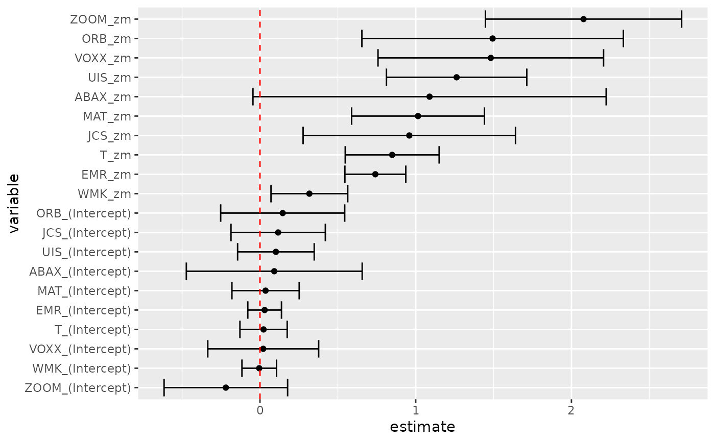
# coefficient plot
library(ggplot2)
library(dplyr)
tidy(res, conf.int = TRUE) |>
mutate(variable = reorder(term, estimate)) |>
ggplot(aes(estimate, variable)) +
geom_point() +
geom_errorbarh(aes(xmin = conf.low, xmax = conf.high)) +
geom_vline(xintercept = 0, color = "red", lty = 2)
 # from a function instead of a matrix
g <- function(theta, x) {
e <- x[, 2:11] - theta[1] - (x[, 1] - theta[1]) %*% matrix(theta[2:11], 1, 10)
gmat <- cbind(e, e * c(x[, 1]))
return(gmat)
}
x <- as.matrix(cbind(rm, r))
res_black <- gmm(g, x = x, t0 = rep(0, 11))
tidy(res_black)
#> # A tibble: 11 × 5
#> term estimate std.error statistic p.value
#> <chr> <dbl> <dbl> <dbl> <dbl>
#> 1 Theta[1] 0.516 0.172 3.00 2.72e- 3
#> 2 Theta[2] 1.12 0.116 9.65 5.02e-22
#> 3 Theta[3] 0.680 0.197 3.45 5.65e- 4
#> 4 Theta[4] -0.0322 0.424 -0.0761 9.39e- 1
#> 5 Theta[5] 0.850 0.155 5.49 4.05e- 8
#> 6 Theta[6] -0.205 0.479 -0.429 6.68e- 1
#> 7 Theta[7] 0.625 0.122 5.14 2.73e- 7
#> 8 Theta[8] 1.05 0.0687 15.3 5.03e-53
#> 9 Theta[9] 0.640 0.233 2.75 5.92e- 3
#> 10 Theta[10] 0.596 0.295 2.02 4.36e- 2
#> 11 Theta[11] 1.16 0.240 4.82 1.45e- 6
tidy(res_black, conf.int = TRUE)
#> # A tibble: 11 × 7
#> term estimate std.error statistic p.value conf.low conf.high
#> <chr> <dbl> <dbl> <dbl> <dbl> <dbl> <dbl>
#> 1 Theta[1] 0.516 0.172 3.00 2.72e- 3 0.178 0.853
#> 2 Theta[2] 1.12 0.116 9.65 5.02e-22 0.889 1.34
#> 3 Theta[3] 0.680 0.197 3.45 5.65e- 4 0.293 1.07
#> 4 Theta[4] -0.0322 0.424 -0.0761 9.39e- 1 -0.862 0.798
#> 5 Theta[5] 0.850 0.155 5.49 4.05e- 8 0.546 1.15
#> 6 Theta[6] -0.205 0.479 -0.429 6.68e- 1 -1.14 0.733
#> 7 Theta[7] 0.625 0.122 5.14 2.73e- 7 0.387 0.864
#> 8 Theta[8] 1.05 0.0687 15.3 5.03e-53 0.919 1.19
#> 9 Theta[9] 0.640 0.233 2.75 5.92e- 3 0.184 1.10
#> 10 Theta[10] 0.596 0.295 2.02 4.36e- 2 0.0171 1.17
#> 11 Theta[11] 1.16 0.240 4.82 1.45e- 6 0.686 1.63
# APT test with Fama-French factors and GMM
f1 <- zm
f2 <- Finance[1:300, "hml"] - rf
f3 <- Finance[1:300, "smb"] - rf
h <- cbind(f1, f2, f3)
res2 <- gmm(z ~ f1 + f2 + f3, x = h)
td2 <- tidy(res2, conf.int = TRUE)
td2
#> # A tibble: 40 × 7
#> term estimate std.error statistic p.value conf.low conf.high
#> <chr> <dbl> <dbl> <dbl> <dbl> <dbl> <dbl>
#> 1 WMK_(Interc… -0.0240 0.0548 -0.438 0.662 -0.131 0.0834
#> 2 UIS_(Interc… 0.0723 0.127 0.567 0.570 -0.177 0.322
#> 3 ORB_(Interc… 0.114 0.212 0.534 0.593 -0.303 0.530
#> 4 MAT_(Interc… 0.0694 0.0979 0.709 0.478 -0.122 0.261
#> 5 ABAX_(Inter… 0.0668 0.275 0.242 0.808 -0.473 0.606
#> 6 T_(Intercep… 0.0195 0.0745 0.262 0.793 -0.126 0.165
#> 7 EMR_(Interc… 0.0217 0.0538 0.404 0.687 -0.0837 0.127
#> 8 JCS_(Interc… 0.0904 0.154 0.586 0.558 -0.212 0.393
#> 9 VOXX_(Inter… -0.00706 0.179 -0.0394 0.969 -0.359 0.344
#> 10 ZOOM_(Inter… -0.189 0.215 -0.878 0.380 -0.610 0.233
#> # ℹ 30 more rows
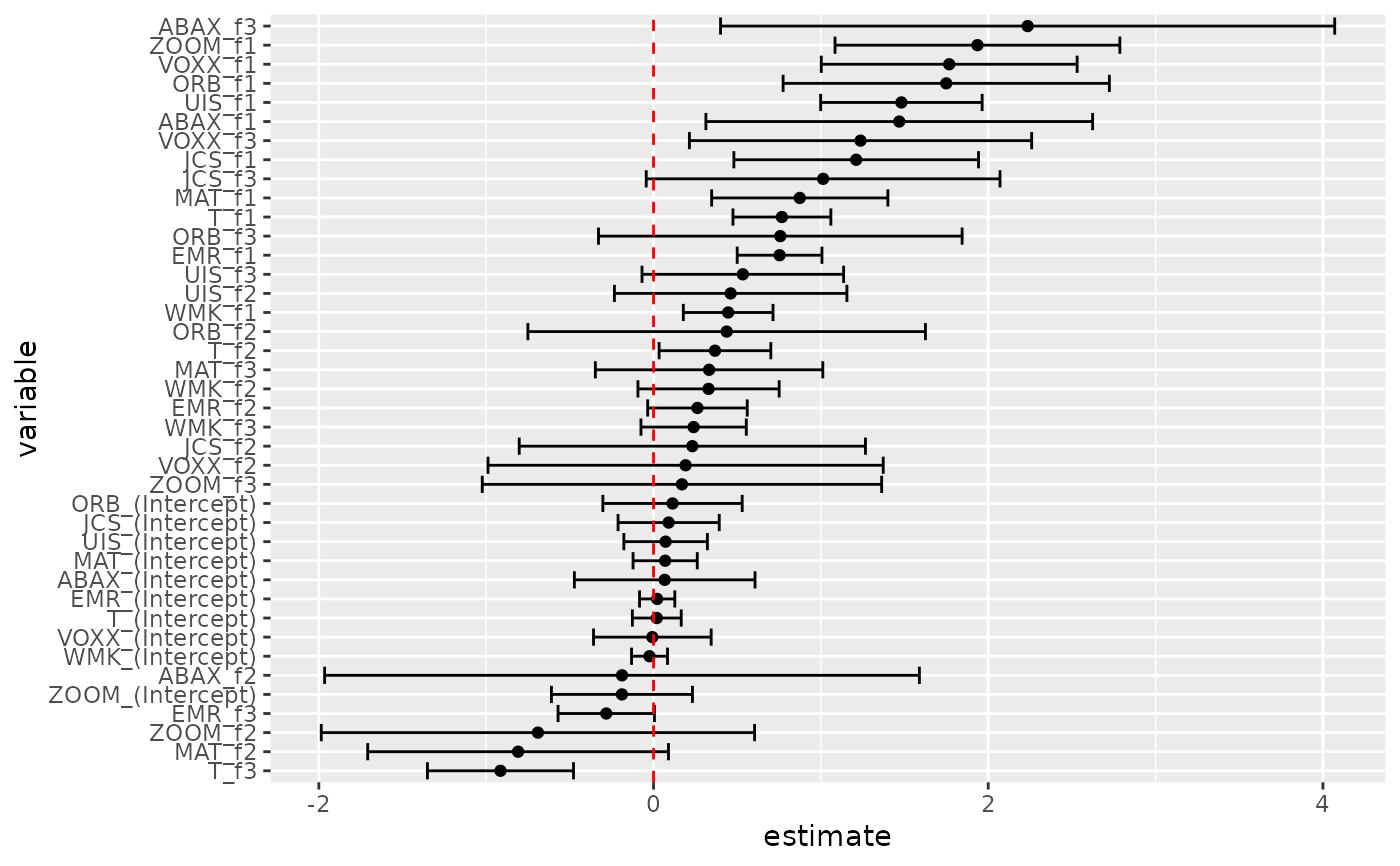
# coefficient plot
td2 |>
mutate(variable = reorder(term, estimate)) |>
ggplot(aes(estimate, variable)) +
geom_point() +
geom_errorbarh(aes(xmin = conf.low, xmax = conf.high)) +
geom_vline(xintercept = 0, color = "red", lty = 2)
# from a function instead of a matrix
g <- function(theta, x) {
e <- x[, 2:11] - theta[1] - (x[, 1] - theta[1]) %*% matrix(theta[2:11], 1, 10)
gmat <- cbind(e, e * c(x[, 1]))
return(gmat)
}
x <- as.matrix(cbind(rm, r))
res_black <- gmm(g, x = x, t0 = rep(0, 11))
tidy(res_black)
#> # A tibble: 11 × 5
#> term estimate std.error statistic p.value
#> <chr> <dbl> <dbl> <dbl> <dbl>
#> 1 Theta[1] 0.516 0.172 3.00 2.72e- 3
#> 2 Theta[2] 1.12 0.116 9.65 5.02e-22
#> 3 Theta[3] 0.680 0.197 3.45 5.65e- 4
#> 4 Theta[4] -0.0322 0.424 -0.0761 9.39e- 1
#> 5 Theta[5] 0.850 0.155 5.49 4.05e- 8
#> 6 Theta[6] -0.205 0.479 -0.429 6.68e- 1
#> 7 Theta[7] 0.625 0.122 5.14 2.73e- 7
#> 8 Theta[8] 1.05 0.0687 15.3 5.03e-53
#> 9 Theta[9] 0.640 0.233 2.75 5.92e- 3
#> 10 Theta[10] 0.596 0.295 2.02 4.36e- 2
#> 11 Theta[11] 1.16 0.240 4.82 1.45e- 6
tidy(res_black, conf.int = TRUE)
#> # A tibble: 11 × 7
#> term estimate std.error statistic p.value conf.low conf.high
#> <chr> <dbl> <dbl> <dbl> <dbl> <dbl> <dbl>
#> 1 Theta[1] 0.516 0.172 3.00 2.72e- 3 0.178 0.853
#> 2 Theta[2] 1.12 0.116 9.65 5.02e-22 0.889 1.34
#> 3 Theta[3] 0.680 0.197 3.45 5.65e- 4 0.293 1.07
#> 4 Theta[4] -0.0322 0.424 -0.0761 9.39e- 1 -0.862 0.798
#> 5 Theta[5] 0.850 0.155 5.49 4.05e- 8 0.546 1.15
#> 6 Theta[6] -0.205 0.479 -0.429 6.68e- 1 -1.14 0.733
#> 7 Theta[7] 0.625 0.122 5.14 2.73e- 7 0.387 0.864
#> 8 Theta[8] 1.05 0.0687 15.3 5.03e-53 0.919 1.19
#> 9 Theta[9] 0.640 0.233 2.75 5.92e- 3 0.184 1.10
#> 10 Theta[10] 0.596 0.295 2.02 4.36e- 2 0.0171 1.17
#> 11 Theta[11] 1.16 0.240 4.82 1.45e- 6 0.686 1.63
# APT test with Fama-French factors and GMM
f1 <- zm
f2 <- Finance[1:300, "hml"] - rf
f3 <- Finance[1:300, "smb"] - rf
h <- cbind(f1, f2, f3)
res2 <- gmm(z ~ f1 + f2 + f3, x = h)
td2 <- tidy(res2, conf.int = TRUE)
td2
#> # A tibble: 40 × 7
#> term estimate std.error statistic p.value conf.low conf.high
#> <chr> <dbl> <dbl> <dbl> <dbl> <dbl> <dbl>
#> 1 WMK_(Interc… -0.0240 0.0548 -0.438 0.662 -0.131 0.0834
#> 2 UIS_(Interc… 0.0723 0.127 0.567 0.570 -0.177 0.322
#> 3 ORB_(Interc… 0.114 0.212 0.534 0.593 -0.303 0.530
#> 4 MAT_(Interc… 0.0694 0.0979 0.709 0.478 -0.122 0.261
#> 5 ABAX_(Inter… 0.0668 0.275 0.242 0.808 -0.473 0.606
#> 6 T_(Intercep… 0.0195 0.0745 0.262 0.793 -0.126 0.165
#> 7 EMR_(Interc… 0.0217 0.0538 0.404 0.687 -0.0837 0.127
#> 8 JCS_(Interc… 0.0904 0.154 0.586 0.558 -0.212 0.393
#> 9 VOXX_(Inter… -0.00706 0.179 -0.0394 0.969 -0.359 0.344
#> 10 ZOOM_(Inter… -0.189 0.215 -0.878 0.380 -0.610 0.233
#> # ℹ 30 more rows
# coefficient plot
td2 |>
mutate(variable = reorder(term, estimate)) |>
ggplot(aes(estimate, variable)) +
geom_point() +
geom_errorbarh(aes(xmin = conf.low, xmax = conf.high)) +
geom_vline(xintercept = 0, color = "red", lty = 2)