Glance at a(n) pam object

Glance accepts a model object and returns a tibble::tibble() with exactly one row of model summaries. The summaries are typically goodness of fit measures, p-values for hypothesis tests on residuals, or model convergence information.

Glance never returns information from the original call to the modeling function. This includes the name of the modeling function or any arguments passed to the modeling function.

Glance does not calculate summary measures. Rather, it farms out these computations to appropriate methods and gathers the results together. Sometimes a goodness of fit measure will be undefined. In these cases the measure will be reported as NA.

Glance returns the same number of columns regardless of whether the model matrix is rank-deficient or not. If so, entries in columns that no longer have a well-defined value are filled in with an NA of the appropriate type.

Usage

# S3 method for class 'pam'
glance(x, ...)

Arguments

x

An pam object returned from cluster::pam()

...

Additional arguments. Not used. Needed to match generic signature only. Cautionary note: Misspelled arguments will be absorbed in ..., where they will be ignored. If the misspelled argument has a default value, the default value will be used. For example, if you pass conf.lvel = 0.9, all computation will proceed using conf.level = 0.95. Two exceptions here are:

• tidy() methods will warn when supplied an exponentiate argument if it will be ignored.

• augment() methods will warn when supplied a newdata argument if it will be ignored.

See also

glance(), cluster::pam()

Other pam tidiers: augment.pam(), tidy.pam()

Value

A tibble::tibble() with exactly one row and columns:

avg.silhouette.width

The average silhouette width for the dataset.

Examples

# load libraries for models and data
library(dplyr)
library(ggplot2)
library(cluster)
library(modeldata)
data(hpc_data)

x <- hpc_data[, 2:5]
p <- pam(x, k = 4)

# summarize model fit with tidiers + visualization
tidy(p)
#> # A tibble: 4 × 11
#>    size max.diss avg.diss diameter separation avg.width cluster compounds
#>   <dbl>    <dbl>    <dbl>    <dbl>      <dbl>     <dbl> <fct>       <dbl>
#> 1  3544   13865.     576.   15128.       93.6    0.711  1             242
#> 2   412    3835.    1111.    5704.       93.2    0.398  2             317
#> 3   236    3882.    1317.    5852.       93.2    0.516  3             240
#> 4   139   42999.    5582.   46451.      151.     0.0843 4             724
#> # ℹ 3 more variables: input_fields <dbl>, iterations <dbl>,
#> #   num_pending <dbl>
glance(p)
#> # A tibble: 1 × 1
#>   avg.silhouette.width
#>                  <dbl>
#> 1                0.650
augment(p, x)
#> # A tibble: 4,331 × 5
#>    compounds input_fields iterations num_pending .cluster
#>        <dbl>        <dbl>      <dbl>       <dbl> <fct>   
#>  1       997          137         20           0 1       
#>  2        97          103         20           0 1       
#>  3       101           75         10           0 1       
#>  4        93           76         20           0 1       
#>  5       100           82         20           0 1       
#>  6       100           82         20           0 1       
#>  7       105           88         20           0 1       
#>  8        98           95         20           0 1       
#>  9       101           91         20           0 1       
#> 10        95           92         20           0 1       
#> # ℹ 4,321 more rows

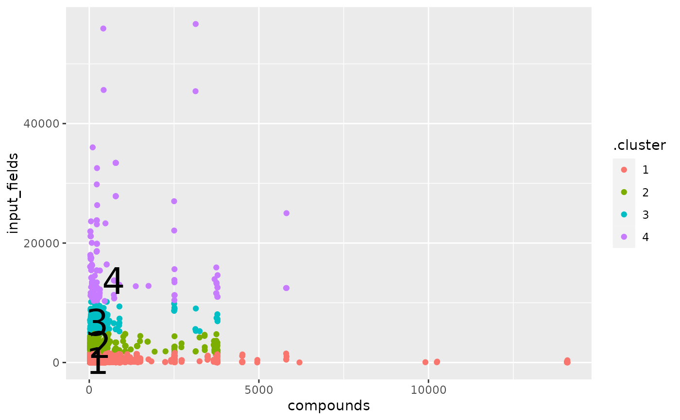
augment(p, x) %>%
  ggplot(aes(compounds, input_fields)) +
  geom_point(aes(color = .cluster)) +
  geom_text(aes(label = cluster), data = tidy(p), size = 10)