Tidy a(n) pam object

Tidy summarizes information about the components of a model. A model component might be a single term in a regression, a single hypothesis, a cluster, or a class. Exactly what tidy considers to be a model component varies across models but is usually self-evident. If a model has several distinct types of components, you will need to specify which components to return.

Usage

# S3 method for class 'pam'
tidy(x, col.names = paste0("x", 1:ncol(x$medoids)), ...)

Arguments

x

An pam object returned from cluster::pam()

col.names

Column names in the input data frame. Defaults to the names of the variables in x.

...

Additional arguments. Not used. Needed to match generic signature only. Cautionary note: Misspelled arguments will be absorbed in ..., where they will be ignored. If the misspelled argument has a default value, the default value will be used. For example, if you pass conf.lvel = 0.9, all computation will proceed using conf.level = 0.95. Two exceptions here are:

• tidy() methods will warn when supplied an exponentiate argument if it will be ignored.

• augment() methods will warn when supplied a newdata argument if it will be ignored.

Details

For examples, see the pam vignette.

See also

tidy(), cluster::pam()

Other pam tidiers: augment.pam(), glance.pam()

Value

A tibble::tibble() with columns:

size

Size of each cluster.

max.diss

Maximal dissimilarity between the observations in the cluster and that cluster's medoid.

avg.diss

Average dissimilarity between the observations in the cluster and that cluster's medoid.

diameter

Diameter of the cluster.

separation

Separation of the cluster.

avg.width

Average silhouette width of the cluster.

cluster

A factor describing the cluster from 1:k.

Examples

# load libraries for models and data
library(dplyr)
library(ggplot2)
library(cluster)
library(modeldata)
data(hpc_data)

x <- hpc_data[, 2:5]
p <- pam(x, k = 4)

# summarize model fit with tidiers + visualization
tidy(p)
#> # A tibble: 4 × 11
#>    size max.diss avg.diss diameter separation avg.width cluster compounds
#>   <dbl>    <dbl>    <dbl>    <dbl>      <dbl>     <dbl> <fct>       <dbl>
#> 1  3544   13865.     576.   15128.       93.6    0.711  1             242
#> 2   412    3835.    1111.    5704.       93.2    0.398  2             317
#> 3   236    3882.    1317.    5852.       93.2    0.516  3             240
#> 4   139   42999.    5582.   46451.      151.     0.0843 4             724
#> # ℹ 3 more variables: input_fields <dbl>, iterations <dbl>,
#> #   num_pending <dbl>
glance(p)
#> # A tibble: 1 × 1
#>   avg.silhouette.width
#>                  <dbl>
#> 1                0.650
augment(p, x)
#> # A tibble: 4,331 × 5
#>    compounds input_fields iterations num_pending .cluster
#>        <dbl>        <dbl>      <dbl>       <dbl> <fct>   
#>  1       997          137         20           0 1       
#>  2        97          103         20           0 1       
#>  3       101           75         10           0 1       
#>  4        93           76         20           0 1       
#>  5       100           82         20           0 1       
#>  6       100           82         20           0 1       
#>  7       105           88         20           0 1       
#>  8        98           95         20           0 1       
#>  9       101           91         20           0 1       
#> 10        95           92         20           0 1       
#> # ℹ 4,321 more rows

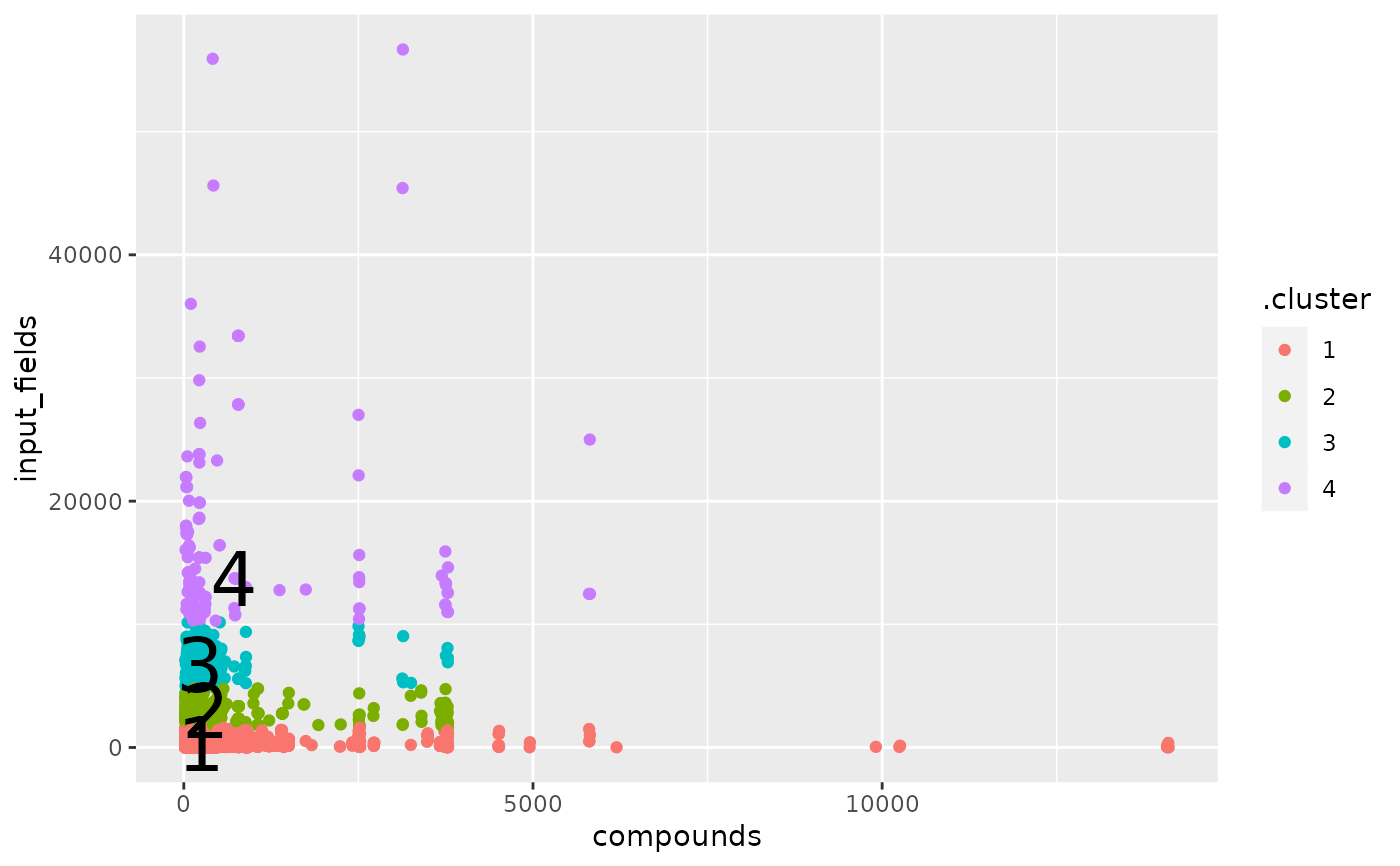
augment(p, x) %>%
  ggplot(aes(compounds, input_fields)) +
  geom_point(aes(color = .cluster)) +
  geom_text(aes(label = cluster), data = tidy(p), size = 10)