Glance at a(n) ridgelm object

Glance accepts a model object and returns a tibble::tibble() with exactly one row of model summaries. The summaries are typically goodness of fit measures, p-values for hypothesis tests on residuals, or model convergence information.

Glance never returns information from the original call to the modeling function. This includes the name of the modeling function or any arguments passed to the modeling function.

Glance does not calculate summary measures. Rather, it farms out these computations to appropriate methods and gathers the results together. Sometimes a goodness of fit measure will be undefined. In these cases the measure will be reported as NA.

Glance returns the same number of columns regardless of whether the model matrix is rank-deficient or not. If so, entries in columns that no longer have a well-defined value are filled in with an NA of the appropriate type.

Usage

# S3 method for ridgelm
glance(x, ...)

Arguments

x

A ridgelm object returned from MASS::lm.ridge().

...

Additional arguments. Not used. Needed to match generic signature only. Cautionary note: Misspelled arguments will be absorbed in ..., where they will be ignored. If the misspelled argument has a default value, the default value will be used. For example, if you pass conf.lvel = 0.9, all computation will proceed using conf.level = 0.95. Two exceptions here are:

• tidy() methods will warn when supplied an exponentiate argument if it will be ignored.

• augment() methods will warn when supplied a newdata argument if it will be ignored.

Details

This is similar to the output of select.ridgelm, but it is returned rather than printed.

See also

glance(), MASS::select.ridgelm(), MASS::lm.ridge()

Other ridgelm tidiers: tidy.ridgelm()

Value

A tibble::tibble() with exactly one row and columns:

kHKB

modified HKB estimate of the ridge constant

kLW

modified L-W estimate of the ridge constant

lambdaGCV

choice of lambda that minimizes GCV

Examples

# load libraries for models and data
library(MASS)

names(longley)[1] <- "y"

# fit model and summarizd results
fit1 <- lm.ridge(y ~ ., longley)
tidy(fit1)
#> # A tibble: 6 × 5
#>   lambda   GCV term         estimate scale
#>    <dbl> <dbl> <chr>           <dbl> <dbl>
#> 1      0 0.128 GNP            25.4   96.2 
#> 2      0 0.128 Unemployed      3.30  90.5 
#> 3      0 0.128 Armed.Forces    0.752 67.4 
#> 4      0 0.128 Population    -11.7    6.74
#> 5      0 0.128 Year           -6.54   4.61
#> 6      0 0.128 Employed        0.786  3.40

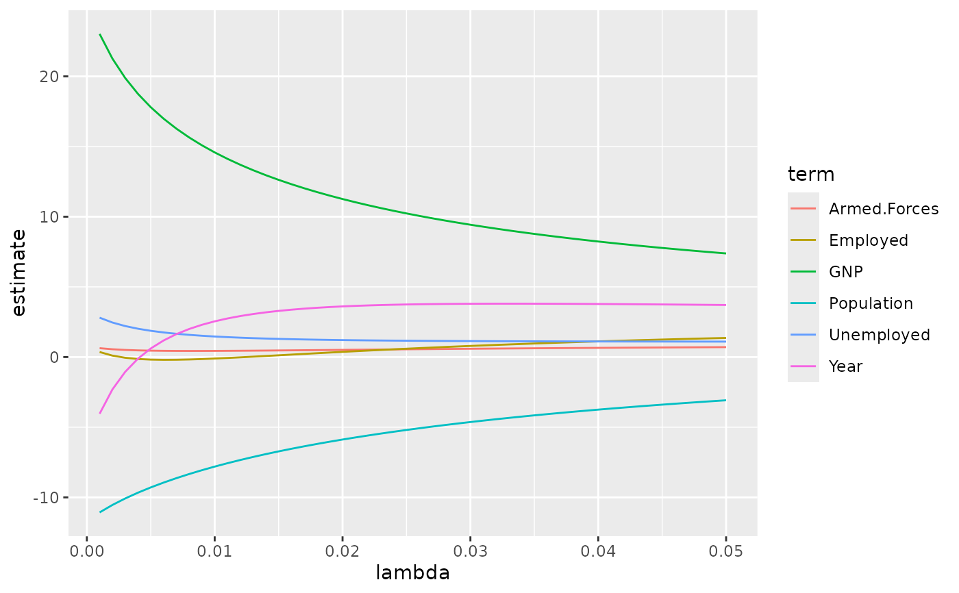
fit2 <- lm.ridge(y ~ ., longley, lambda = seq(0.001, .05, .001))
td2 <- tidy(fit2)
g2 <- glance(fit2)

# coefficient plot
library(ggplot2)
ggplot(td2, aes(lambda, estimate, color = term)) +
  geom_line()


# GCV plot
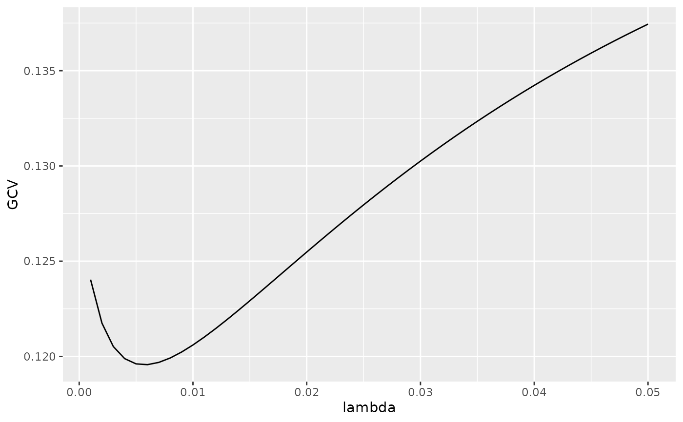
ggplot(td2, aes(lambda, GCV)) +
  geom_line()


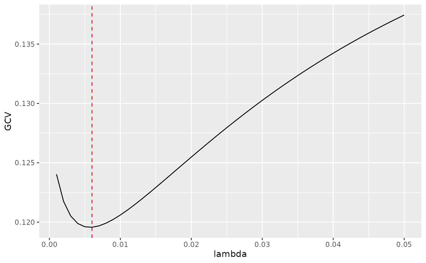
# add line for the GCV minimizing estimate
ggplot(td2, aes(lambda, GCV)) +
  geom_line() +
  geom_vline(xintercept = g2$lambdaGCV, col = "red", lty = 2)