Tidy a(n) ridgelm object

Tidy summarizes information about the components of a model. A model component might be a single term in a regression, a single hypothesis, a cluster, or a class. Exactly what tidy considers to be a model component varies across models but is usually self-evident. If a model has several distinct types of components, you will need to specify which components to return.

Usage

# S3 method for ridgelm
tidy(x, ...)

Arguments

x

A ridgelm object returned from MASS::lm.ridge().

...

Additional arguments. Not used. Needed to match generic signature only. Cautionary note: Misspelled arguments will be absorbed in ..., where they will be ignored. If the misspelled argument has a default value, the default value will be used. For example, if you pass conf.lvel = 0.9, all computation will proceed using conf.level = 0.95. Two exceptions here are:

• tidy() methods will warn when supplied an exponentiate argument if it will be ignored.

• augment() methods will warn when supplied a newdata argument if it will be ignored.

See also

tidy(), MASS::lm.ridge()

Other ridgelm tidiers: glance.ridgelm()

Value

A tibble::tibble() with columns:

GCV

Generalized cross validation error estimate.

lambda

Value of penalty parameter lambda.

term

The name of the regression term.

estimate

estimate of scaled coefficient using this lambda

scale

Scaling factor of estimated coefficient

Examples

# load libraries for models and data
library(MASS)

names(longley)[1] <- "y"

# fit model and summarizd results
fit1 <- lm.ridge(y ~ ., longley)
tidy(fit1)
#> # A tibble: 6 × 5
#>   lambda   GCV term         estimate scale
#>    <dbl> <dbl> <chr>           <dbl> <dbl>
#> 1      0 0.128 GNP            25.4   96.2 
#> 2      0 0.128 Unemployed      3.30  90.5 
#> 3      0 0.128 Armed.Forces    0.752 67.4 
#> 4      0 0.128 Population    -11.7    6.74
#> 5      0 0.128 Year           -6.54   4.61
#> 6      0 0.128 Employed        0.786  3.40

fit2 <- lm.ridge(y ~ ., longley, lambda = seq(0.001, .05, .001))
td2 <- tidy(fit2)
g2 <- glance(fit2)

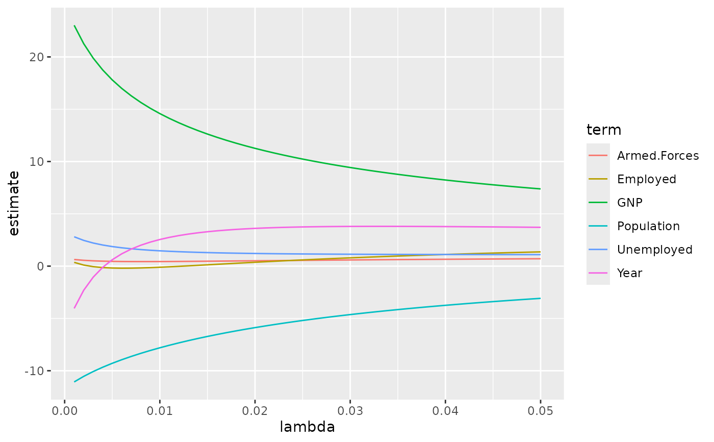
# coefficient plot
library(ggplot2)
ggplot(td2, aes(lambda, estimate, color = term)) +
  geom_line()


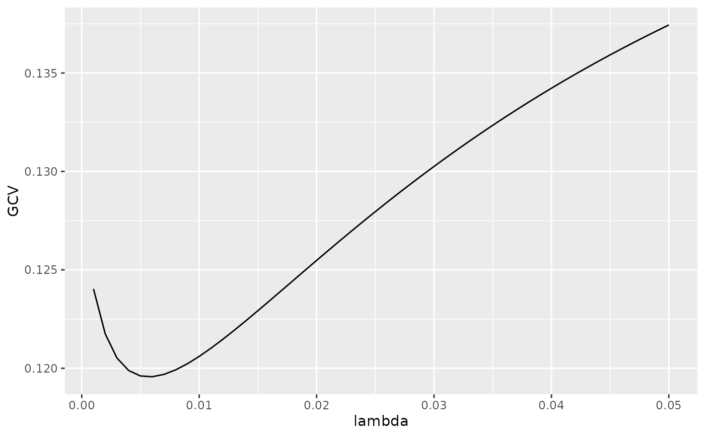
# GCV plot
ggplot(td2, aes(lambda, GCV)) +
  geom_line()


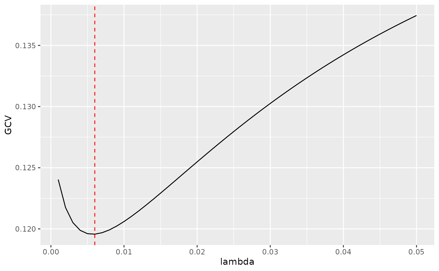
# add line for the GCV minimizing estimate
ggplot(td2, aes(lambda, GCV)) +
  geom_line() +
  geom_vline(xintercept = g2$lambdaGCV, col = "red", lty = 2)