Tidy a(n) cv.glmnet object

Tidy summarizes information about the components of a model. A model component might be a single term in a regression, a single hypothesis, a cluster, or a class. Exactly what tidy considers to be a model component varies across models but is usually self-evident. If a model has several distinct types of components, you will need to specify which components to return.

Usage

# S3 method for cv.glmnet
tidy(x, ...)

Arguments

x

A cv.glmnet object returned from glmnet::cv.glmnet().

...

Additional arguments. Not used. Needed to match generic signature only. Cautionary note: Misspelled arguments will be absorbed in ..., where they will be ignored. If the misspelled argument has a default value, the default value will be used. For example, if you pass conf.lvel = 0.9, all computation will proceed using conf.level = 0.95. Two exceptions here are:

tidy() methods will warn when supplied an exponentiate argument if it will be ignored.
augment() methods will warn when supplied a newdata argument if it will be ignored.

Value

A tibble::tibble() with columns:

lambda: Value of penalty parameter lambda.
nzero: Number of non-zero coefficients for the given lambda.
std.error: The standard error of the regression term.
conf.low: lower bound on confidence interval for cross-validation estimated loss.
conf.high: upper bound on confidence interval for cross-validation estimated loss.
estimate: Median loss across all cross-validation folds for a given lamdba

Examples


# load libraries for models and data
library(glmnet)

set.seed(27)

nobs <- 100
nvar <- 50
real <- 5

x <- matrix(rnorm(nobs * nvar), nobs, nvar)
beta <- c(rnorm(real, 0, 1), rep(0, nvar - real))
y <- c(t(beta) %*% t(x)) + rnorm(nvar, sd = 3)

cvfit1 <- cv.glmnet(x, y)

tidy(cvfit1)
#> # A tibble: 74 × 6
#>    lambda estimate std.error conf.low conf.high nzero
#>     <dbl>    <dbl>     <dbl>    <dbl>     <dbl> <int>
#>  1  1.45      17.4      2.28     15.1      19.7     0
#>  2  1.32      17.4      2.28     15.1      19.7     1
#>  3  1.20      17.2      2.22     15.0      19.5     1
#>  4  1.09      17.0      2.15     14.8      19.1     1
#>  5  0.997     16.8      2.09     14.7      18.9     1
#>  6  0.909     16.7      2.03     14.7      18.7     2
#>  7  0.828     16.7      1.99     14.7      18.6     3
#>  8  0.754     16.7      1.95     14.7      18.6     5
#>  9  0.687     16.8      1.93     14.8      18.7     7
#> 10  0.626     16.9      1.91     15.0      18.8     7
#> # ℹ 64 more rows
glance(cvfit1)
#> # A tibble: 1 × 3
#>   lambda.min lambda.1se  nobs
#>        <dbl>      <dbl> <int>
#> 1      0.828       1.45   100

library(ggplot2)

tidied_cv <- tidy(cvfit1)
glance_cv <- glance(cvfit1)

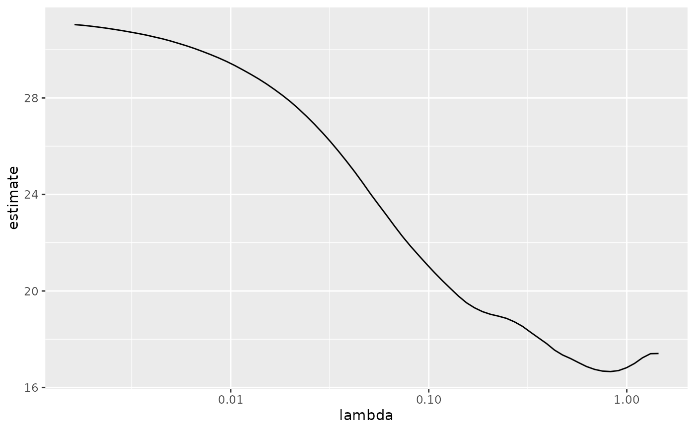
# plot of MSE as a function of lambda
g <- ggplot(tidied_cv, aes(lambda, estimate)) +
  geom_line() +
  scale_x_log10()
g


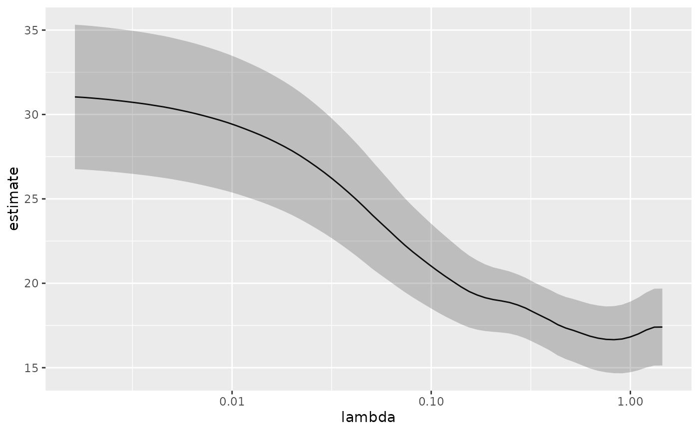
# plot of MSE as a function of lambda with confidence ribbon
g <- g + geom_ribbon(aes(ymin = conf.low, ymax = conf.high), alpha = .25)
g


# plot of MSE as a function of lambda with confidence ribbon and choices
# of minimum lambda marked
g <- g +
  geom_vline(xintercept = glance_cv$lambda.min) +
  geom_vline(xintercept = glance_cv$lambda.1se, lty = 2)
g


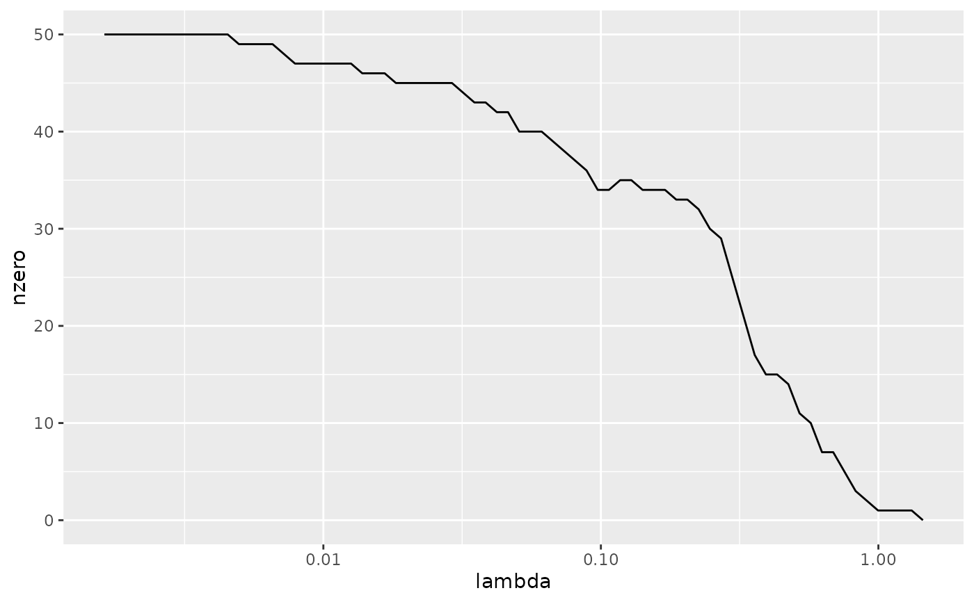
# plot of number of zeros for each choice of lambda
ggplot(tidied_cv, aes(lambda, nzero)) +
  geom_line() +
  scale_x_log10()


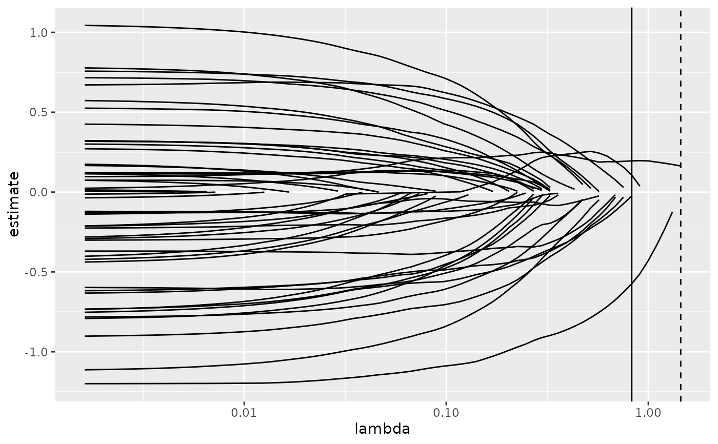
# coefficient plot with min lambda shown
tidied <- tidy(cvfit1$glmnet.fit)

ggplot(tidied, aes(lambda, estimate, group = term)) +
  scale_x_log10() +
  geom_line() +
  geom_vline(xintercept = glance_cv$lambda.min) +
  geom_vline(xintercept = glance_cv$lambda.1se, lty = 2)

Usage

Arguments

See also

Value

Examples