Tidy a(n) poLCA object

Tidy summarizes information about the components of a model. A model component might be a single term in a regression, a single hypothesis, a cluster, or a class. Exactly what tidy considers to be a model component varies across models but is usually self-evident. If a model has several distinct types of components, you will need to specify which components to return.

Usage

# S3 method for poLCA
tidy(x, ...)

Arguments

x

A poLCA object returned from poLCA::poLCA().

...

Additional arguments. Not used. Needed to match generic signature only. Cautionary note: Misspelled arguments will be absorbed in ..., where they will be ignored. If the misspelled argument has a default value, the default value will be used. For example, if you pass conf.lvel = 0.9, all computation will proceed using conf.level = 0.95. Two exceptions here are:

tidy() methods will warn when supplied an exponentiate argument if it will be ignored.
augment() methods will warn when supplied a newdata argument if it will be ignored.

Value

A tibble::tibble() with columns:

class: The class under consideration.
outcome: Outcome of manifest variable.
std.error: The standard error of the regression term.
variable: Manifest variable
estimate: Estimated class-conditional response probability

Examples


# load libraries for models and data
library(poLCA)
library(dplyr)

# generate data
data(values)

f <- cbind(A, B, C, D) ~ 1

# fit model
M1 <- poLCA(f, values, nclass = 2, verbose = FALSE)

M1
#> Conditional item response (column) probabilities,
#>  by outcome variable, for each class (row) 
#>  
#> $A
#>            Pr(1)  Pr(2)
#> class 1:  0.2864 0.7136
#> class 2:  0.0068 0.9932
#> 
#> $B
#>            Pr(1)  Pr(2)
#> class 1:  0.6704 0.3296
#> class 2:  0.0602 0.9398
#> 
#> $C
#>            Pr(1)  Pr(2)
#> class 1:  0.6460 0.3540
#> class 2:  0.0735 0.9265
#> 
#> $D
#>            Pr(1)  Pr(2)
#> class 1:  0.8676 0.1324
#> class 2:  0.2309 0.7691
#> 
#> Estimated class population shares 
#>  0.7208 0.2792 
#>  
#> Predicted class memberships (by modal posterior prob.) 
#>  0.6713 0.3287 
#>  
#> ========================================================= 
#> Fit for 2 latent classes: 
#> ========================================================= 
#> number of observations: 216 
#> number of estimated parameters: 9 
#> residual degrees of freedom: 6 
#> maximum log-likelihood: -504.4677 
#>  
#> AIC(2): 1026.935
#> BIC(2): 1057.313
#> G^2(2): 2.719922 (Likelihood ratio/deviance statistic) 
#> X^2(2): 2.719764 (Chi-square goodness of fit) 
#>  

# summarize model fit with tidiers + visualization
tidy(M1)
#> # A tibble: 16 × 5
#>    variable class outcome estimate std.error
#>    <chr>    <int>   <dbl>    <dbl>     <dbl>
#>  1 A            1       1  0.286      0.0393
#>  2 A            2       1  0.00681    0.0254
#>  3 A            1       2  0.714      0.0393
#>  4 A            2       2  0.993      0.0254
#>  5 B            1       1  0.670      0.0489
#>  6 B            2       1  0.0602     0.0649
#>  7 B            1       2  0.330      0.0489
#>  8 B            2       2  0.940      0.0649
#>  9 C            1       1  0.646      0.0482
#> 10 C            2       1  0.0735     0.0642
#> 11 C            1       2  0.354      0.0482
#> 12 C            2       2  0.927      0.0642
#> 13 D            1       1  0.868      0.0379
#> 14 D            2       1  0.231      0.0929
#> 15 D            1       2  0.132      0.0379
#> 16 D            2       2  0.769      0.0929
augment(M1)
#> # A tibble: 216 × 7
#>        A     B     C     D X.Intercept. .class .probability
#>    <dbl> <dbl> <dbl> <dbl>        <dbl>  <int>        <dbl>
#>  1     2     2     2     2            1      2        0.959
#>  2     2     2     2     2            1      2        0.959
#>  3     2     2     2     2            1      2        0.959
#>  4     2     2     2     2            1      2        0.959
#>  5     2     2     2     2            1      2        0.959
#>  6     2     2     2     2            1      2        0.959
#>  7     2     2     2     2            1      2        0.959
#>  8     2     2     2     2            1      2        0.959
#>  9     2     2     2     2            1      2        0.959
#> 10     2     2     2     2            1      2        0.959
#> # ℹ 206 more rows
glance(M1)
#> # A tibble: 1 × 8
#>   logLik   AIC   BIC g.squared chi.squared    df df.residual  nobs
#>    <dbl> <dbl> <dbl>     <dbl>       <dbl> <dbl>       <dbl> <int>
#> 1  -504. 1027. 1057.      2.72        2.72     9           6   216

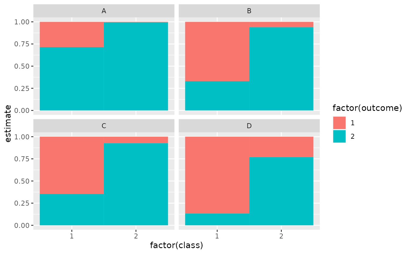
library(ggplot2)

ggplot(tidy(M1), aes(factor(class), estimate, fill = factor(outcome))) +
  geom_bar(stat = "identity", width = 1) +
  facet_wrap(~variable)


# three-class model with a single covariate.
data(election)

f2a <- cbind(
  MORALG, CARESG, KNOWG, LEADG, DISHONG, INTELG,
  MORALB, CARESB, KNOWB, LEADB, DISHONB, INTELB
) ~ PARTY

nes2a <- poLCA(f2a, election, nclass = 3, nrep = 5, verbose = FALSE)
#> Error in eval(predvars, data, env): object 'MORALG' not found

td <- tidy(nes2a)
#> Error in eval(expr, envir, enclos): object 'nes2a' not found
td
#> Error in eval(expr, envir, enclos): object 'td' not found

ggplot(td, aes(outcome, estimate, color = factor(class), group = class)) +
  geom_line() +
  facet_wrap(~variable, nrow = 2) +
  theme(axis.text.x = element_text(angle = 90, hjust = 1))
#> Error in eval(expr, envir, enclos): object 'td' not found

au <- augment(nes2a)
#> Error in eval(expr, envir, enclos): object 'nes2a' not found

au
#> Error in eval(expr, envir, enclos): object 'au' not found

count(au, .class)
#> Error in eval(expr, envir, enclos): object 'au' not found

# if the original data is provided, it leads to NAs in new columns
# for rows that weren't predicted
au2 <- augment(nes2a, data = election)
#> Error in eval(expr, envir, enclos): object 'nes2a' not found

au2
#> Error in eval(expr, envir, enclos): object 'au2' not found

dim(au2)
#> Error in eval(expr, envir, enclos): object 'au2' not found

Usage

Arguments

See also

Value

Examples