Tidy summarizes information about the components of a model. A model component might be a single term in a regression, a single hypothesis, a cluster, or a class. Exactly what tidy considers to be a model component varies across models but is usually self-evident. If a model has several distinct types of components, you will need to specify which components to return.
Usage
# S3 method for class 'summary.glht'
tidy(x, ...)
Arguments
- x
A
summary.glhtobject created by callingmultcomp::summary.glht()on aglhtobject created withmultcomp::glht().- ...
Additional arguments. Not used. Needed to match generic signature only. Cautionary note: Misspelled arguments will be absorbed in
..., where they will be ignored. If the misspelled argument has a default value, the default value will be used. For example, if you passconf.lvel = 0.9, all computation will proceed usingconf.level = 0.95. Two exceptions here are:
See also
tidy(), multcomp::summary.glht(), multcomp::glht()
Other multcomp tidiers:
tidy.cld(),
tidy.confint.glht(),
tidy.glht()
Value
A tibble::tibble() with columns:
- contrast
Levels being compared.
- estimate
The estimated value of the regression term.
- null.value
Value to which the estimate is compared.
- p.value
The two-sided p-value associated with the observed statistic.
- statistic
The value of a T-statistic to use in a hypothesis that the regression term is non-zero.
- std.error
The standard error of the regression term.
Examples
# load libraries for models and data
library(multcomp)
library(ggplot2)
amod <- aov(breaks ~ wool + tension, data = warpbreaks)
wht <- glht(amod, linfct = mcp(tension = "Tukey"))
tidy(wht)
#> # A tibble: 3 × 7
#> term contrast null.value estimate std.error statistic adj.p.value
#> <chr> <chr> <dbl> <dbl> <dbl> <dbl> <dbl>
#> 1 tension M - L 0 -10 3.87 -2.58 0.0337
#> 2 tension H - L 0 -14.7 3.87 -3.80 0.00109
#> 3 tension H - M 0 -4.72 3.87 -1.22 0.447
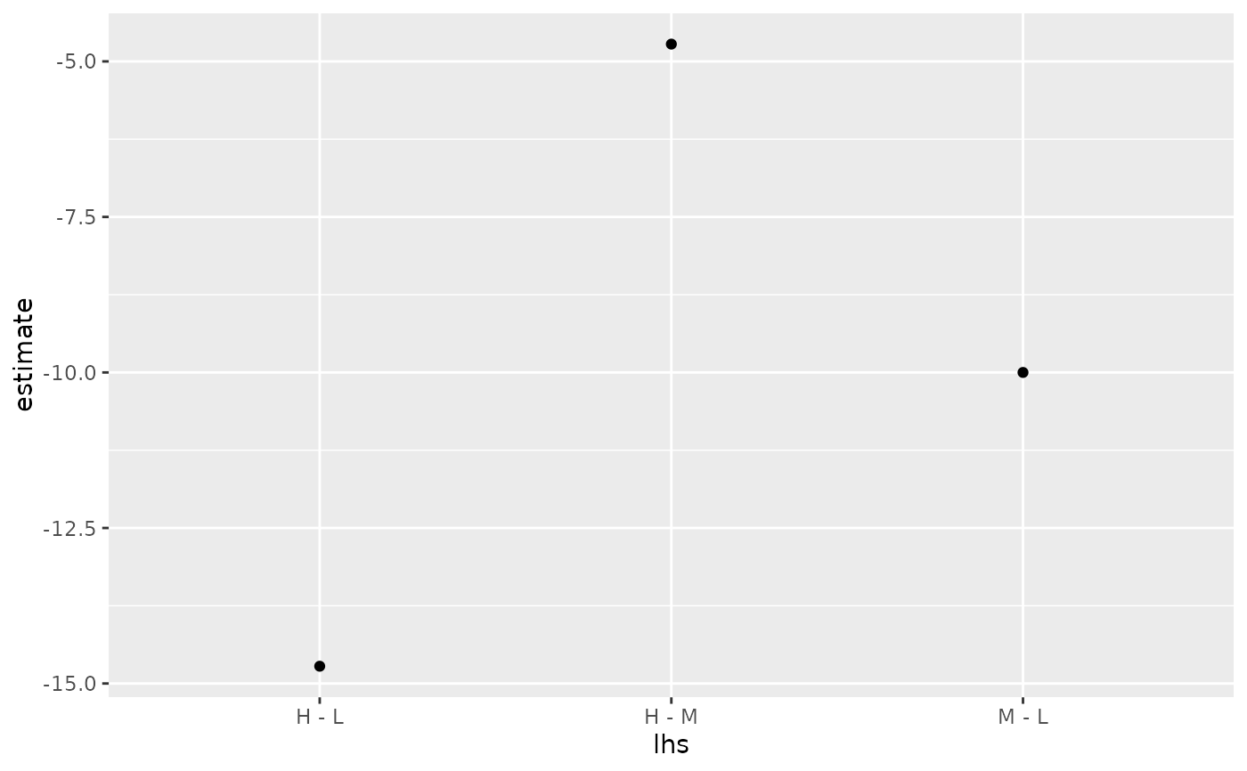
ggplot(wht, aes(lhs, estimate)) +
geom_point()
 CI <- confint(wht)
tidy(CI)
#> # A tibble: 3 × 5
#> term contrast estimate conf.low conf.high
#> <chr> <chr> <dbl> <dbl> <dbl>
#> 1 tension M - L -10 -19.4 -0.643
#> 2 tension H - L -14.7 -24.1 -5.37
#> 3 tension H - M -4.72 -14.1 4.63
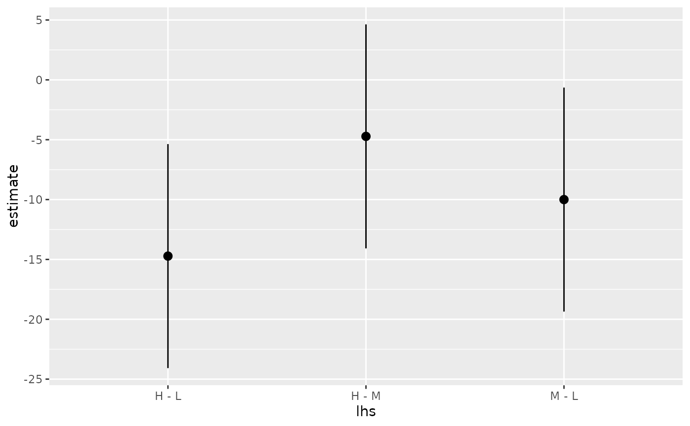
ggplot(CI, aes(lhs, estimate, ymin = lwr, ymax = upr)) +
geom_pointrange()
CI <- confint(wht)
tidy(CI)
#> # A tibble: 3 × 5
#> term contrast estimate conf.low conf.high
#> <chr> <chr> <dbl> <dbl> <dbl>
#> 1 tension M - L -10 -19.4 -0.643
#> 2 tension H - L -14.7 -24.1 -5.37
#> 3 tension H - M -4.72 -14.1 4.63
ggplot(CI, aes(lhs, estimate, ymin = lwr, ymax = upr)) +
geom_pointrange()
 tidy(summary(wht))
#> # A tibble: 3 × 7
#> term contrast null.value estimate std.error statistic adj.p.value
#> <chr> <chr> <dbl> <dbl> <dbl> <dbl> <dbl>
#> 1 tension M - L 0 -10 3.87 -2.58 0.0336
#> 2 tension H - L 0 -14.7 3.87 -3.80 0.00121
#> 3 tension H - M 0 -4.72 3.87 -1.22 0.447
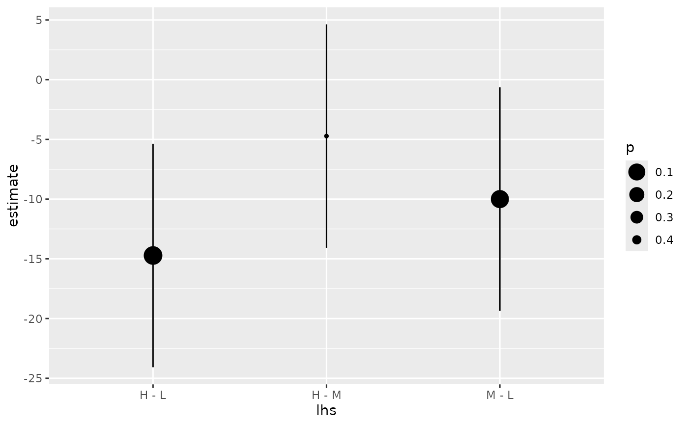
ggplot(mapping = aes(lhs, estimate)) +
geom_linerange(aes(ymin = lwr, ymax = upr), data = CI) +
geom_point(aes(size = p), data = summary(wht)) +
scale_size(trans = "reverse")
tidy(summary(wht))
#> # A tibble: 3 × 7
#> term contrast null.value estimate std.error statistic adj.p.value
#> <chr> <chr> <dbl> <dbl> <dbl> <dbl> <dbl>
#> 1 tension M - L 0 -10 3.87 -2.58 0.0336
#> 2 tension H - L 0 -14.7 3.87 -3.80 0.00121
#> 3 tension H - M 0 -4.72 3.87 -1.22 0.447
ggplot(mapping = aes(lhs, estimate)) +
geom_linerange(aes(ymin = lwr, ymax = upr), data = CI) +
geom_point(aes(size = p), data = summary(wht)) +
scale_size(trans = "reverse")
 cld <- cld(wht)
tidy(cld)
#> # A tibble: 3 × 2
#> tension letters
#> <chr> <chr>
#> 1 L a
#> 2 M b
#> 3 H b
cld <- cld(wht)
tidy(cld)
#> # A tibble: 3 × 2
#> tension letters
#> <chr> <chr>
#> 1 L a
#> 2 M b
#> 3 H b