Glance accepts a model object and returns a tibble::tibble()
with exactly one row of model summaries. The summaries are typically
goodness of fit measures, p-values for hypothesis tests on residuals,
or model convergence information.
Glance never returns information from the original call to the modeling function. This includes the name of the modeling function or any arguments passed to the modeling function.
Glance does not calculate summary measures. Rather, it farms out these
computations to appropriate methods and gathers the results together.
Sometimes a goodness of fit measure will be undefined. In these cases
the measure will be reported as NA.
Glance returns the same number of columns regardless of whether the
model matrix is rank-deficient or not. If so, entries in columns
that no longer have a well-defined value are filled in with an NA
of the appropriate type.
Usage
# S3 method for class 'lm'
glance(x, ...)
Arguments
- x
An
lmobject created bystats::lm().- ...
Additional arguments. Not used. Needed to match generic signature only. Cautionary note: Misspelled arguments will be absorbed in
..., where they will be ignored. If the misspelled argument has a default value, the default value will be used. For example, if you passconf.lvel = 0.9, all computation will proceed usingconf.level = 0.95. Two exceptions here are:
Value
A tibble::tibble() with exactly one row and columns:
- adj.r.squared
Adjusted R squared statistic, which is like the R squared statistic except taking degrees of freedom into account.
- AIC
Akaike's Information Criterion for the model.
- BIC
Bayesian Information Criterion for the model.
- deviance
Deviance of the model.
- df.residual
Residual degrees of freedom.
- logLik
The log-likelihood of the model. [stats::logLik()] may be a useful reference.
- nobs
Number of observations used.
- p.value
P-value corresponding to the test statistic.
- r.squared
R squared statistic, or the percent of variation explained by the model. Also known as the coefficient of determination.
- sigma
Estimated standard error of the residuals.
- statistic
Test statistic.
- df
The degrees for freedom from the numerator of the overall F-statistic. This is new in broom 0.7.0. Previously, this reported the rank of the design matrix, which is one more than the numerator degrees of freedom of the overall F-statistic.
Examples
library(ggplot2)
library(dplyr)
mod <- lm(mpg ~ wt + qsec, data = mtcars)
tidy(mod)
#> # A tibble: 3 × 5
#> term estimate std.error statistic p.value
#> <chr> <dbl> <dbl> <dbl> <dbl>
#> 1 (Intercept) 19.7 5.25 3.76 7.65e- 4
#> 2 wt -5.05 0.484 -10.4 2.52e-11
#> 3 qsec 0.929 0.265 3.51 1.50e- 3
glance(mod)
#> # A tibble: 1 × 12
#> r.squared adj.r.squared sigma statistic p.value df logLik AIC
#> <dbl> <dbl> <dbl> <dbl> <dbl> <dbl> <dbl> <dbl>
#> 1 0.826 0.814 2.60 69.0 9.39e-12 2 -74.4 157.
#> # ℹ 4 more variables: BIC <dbl>, deviance <dbl>, df.residual <int>,
#> # nobs <int>
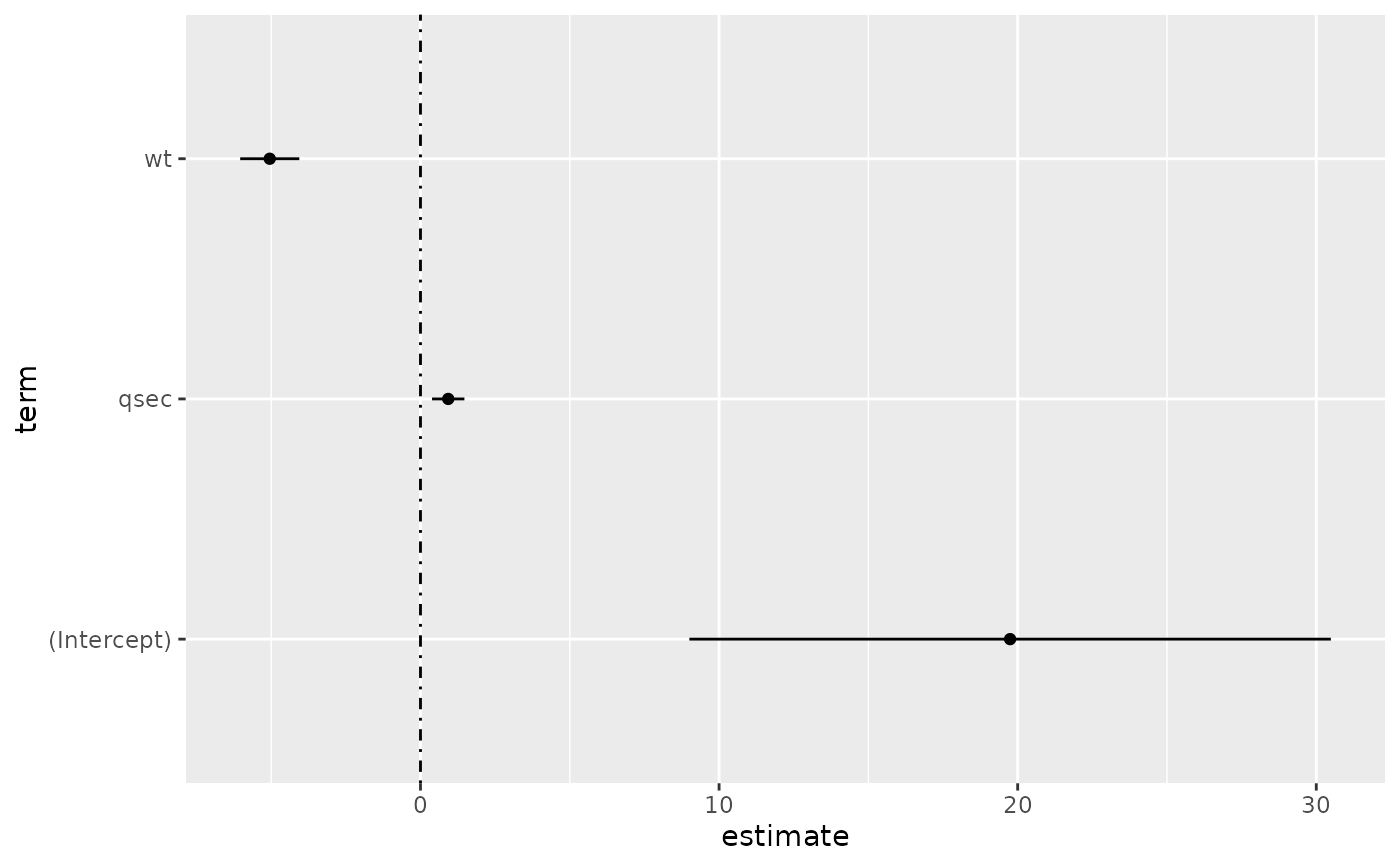
# coefficient plot
d <- tidy(mod, conf.int = TRUE)
ggplot(d, aes(estimate, term, xmin = conf.low, xmax = conf.high, height = 0)) +
geom_point() +
geom_vline(xintercept = 0, lty = 4) +
geom_errorbarh()
 # aside: There are tidy() and glance() methods for lm.summary objects too.
# this can be useful when you want to conserve memory by converting large lm
# objects into their leaner summary.lm equivalents.
s <- summary(mod)
tidy(s, conf.int = TRUE)
#> # A tibble: 3 × 7
#> term estimate std.error statistic p.value conf.low conf.high
#> <chr> <dbl> <dbl> <dbl> <dbl> <dbl> <dbl>
#> 1 (Intercept) 19.7 5.25 3.76 7.65e- 4 9.00 30.5
#> 2 wt -5.05 0.484 -10.4 2.52e-11 -6.04 -4.06
#> 3 qsec 0.929 0.265 3.51 1.50e- 3 0.387 1.47
glance(s)
#> # A tibble: 1 × 8
#> r.squared adj.r.squared sigma statistic p.value df df.residual
#> <dbl> <dbl> <dbl> <dbl> <dbl> <dbl> <int>
#> 1 0.826 0.814 2.60 69.0 9.39e-12 2 29
#> # ℹ 1 more variable: nobs <dbl>
augment(mod)
#> # A tibble: 32 × 10
#> .rownames mpg wt qsec .fitted .resid .hat .sigma .cooksd
#> <chr> <dbl> <dbl> <dbl> <dbl> <dbl> <dbl> <dbl> <dbl>
#> 1 Mazda RX4 21 2.62 16.5 21.8 -0.815 0.0693 2.64 2.63e-3
#> 2 Mazda RX4 W… 21 2.88 17.0 21.0 -0.0482 0.0444 2.64 5.59e-6
#> 3 Datsun 710 22.8 2.32 18.6 25.3 -2.53 0.0607 2.60 2.17e-2
#> 4 Hornet 4 Dr… 21.4 3.22 19.4 21.6 -0.181 0.0576 2.64 1.05e-4
#> 5 Hornet Spor… 18.7 3.44 17.0 18.2 0.504 0.0389 2.64 5.29e-4
#> 6 Valiant 18.1 3.46 20.2 21.1 -2.97 0.0957 2.58 5.10e-2
#> 7 Duster 360 14.3 3.57 15.8 16.4 -2.14 0.0729 2.61 1.93e-2
#> 8 Merc 240D 24.4 3.19 20 22.2 2.17 0.0791 2.61 2.18e-2
#> 9 Merc 230 22.8 3.15 22.9 25.1 -2.32 0.295 2.59 1.59e-1
#> 10 Merc 280 19.2 3.44 18.3 19.4 -0.185 0.0358 2.64 6.55e-5
#> # ℹ 22 more rows
#> # ℹ 1 more variable: .std.resid <dbl>
augment(mod, mtcars, interval = "confidence")
#> # A tibble: 32 × 20
#> .rownames mpg cyl disp hp drat wt qsec vs am
#> <chr> <dbl> <dbl> <dbl> <dbl> <dbl> <dbl> <dbl> <dbl> <dbl>
#> 1 Mazda RX4 21 6 160 110 3.9 2.62 16.5 0 1
#> 2 Mazda RX4 Wag 21 6 160 110 3.9 2.88 17.0 0 1
#> 3 Datsun 710 22.8 4 108 93 3.85 2.32 18.6 1 1
#> 4 Hornet 4 Drive 21.4 6 258 110 3.08 3.22 19.4 1 0
#> 5 Hornet Sporta… 18.7 8 360 175 3.15 3.44 17.0 0 0
#> 6 Valiant 18.1 6 225 105 2.76 3.46 20.2 1 0
#> 7 Duster 360 14.3 8 360 245 3.21 3.57 15.8 0 0
#> 8 Merc 240D 24.4 4 147. 62 3.69 3.19 20 1 0
#> 9 Merc 230 22.8 4 141. 95 3.92 3.15 22.9 1 0
#> 10 Merc 280 19.2 6 168. 123 3.92 3.44 18.3 1 0
#> # ℹ 22 more rows
#> # ℹ 10 more variables: gear <dbl>, carb <dbl>, .fitted <dbl>,
#> # .lower <dbl>, .upper <dbl>, .resid <dbl>, .hat <dbl>,
#> # .sigma <dbl>, .cooksd <dbl>, .std.resid <dbl>
# predict on new data
newdata <- mtcars |>
head(6) |>
mutate(wt = wt + 1)
augment(mod, newdata = newdata)
#> # A tibble: 6 × 14
#> .rownames mpg cyl disp hp drat wt qsec vs am gear
#> <chr> <dbl> <dbl> <dbl> <dbl> <dbl> <dbl> <dbl> <dbl> <dbl> <dbl>
#> 1 Mazda RX4 21 6 160 110 3.9 3.62 16.5 0 1 4
#> 2 Mazda RX… 21 6 160 110 3.9 3.88 17.0 0 1 4
#> 3 Datsun 7… 22.8 4 108 93 3.85 3.32 18.6 1 1 4
#> 4 Hornet 4… 21.4 6 258 110 3.08 4.22 19.4 1 0 3
#> 5 Hornet S… 18.7 8 360 175 3.15 4.44 17.0 0 0 3
#> 6 Valiant 18.1 6 225 105 2.76 4.46 20.2 1 0 3
#> # ℹ 3 more variables: carb <dbl>, .fitted <dbl>, .resid <dbl>
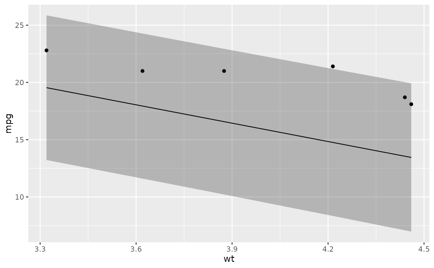
# ggplot2 example where we also construct 95% prediction interval
# simpler bivariate model since we're plotting in 2D
mod2 <- lm(mpg ~ wt, data = mtcars)
au <- augment(mod2, newdata = newdata, interval = "prediction")
ggplot(au, aes(wt, mpg)) +
geom_point() +
geom_line(aes(y = .fitted)) +
geom_ribbon(aes(ymin = .lower, ymax = .upper), col = NA, alpha = 0.3)
# aside: There are tidy() and glance() methods for lm.summary objects too.
# this can be useful when you want to conserve memory by converting large lm
# objects into their leaner summary.lm equivalents.
s <- summary(mod)
tidy(s, conf.int = TRUE)
#> # A tibble: 3 × 7
#> term estimate std.error statistic p.value conf.low conf.high
#> <chr> <dbl> <dbl> <dbl> <dbl> <dbl> <dbl>
#> 1 (Intercept) 19.7 5.25 3.76 7.65e- 4 9.00 30.5
#> 2 wt -5.05 0.484 -10.4 2.52e-11 -6.04 -4.06
#> 3 qsec 0.929 0.265 3.51 1.50e- 3 0.387 1.47
glance(s)
#> # A tibble: 1 × 8
#> r.squared adj.r.squared sigma statistic p.value df df.residual
#> <dbl> <dbl> <dbl> <dbl> <dbl> <dbl> <int>
#> 1 0.826 0.814 2.60 69.0 9.39e-12 2 29
#> # ℹ 1 more variable: nobs <dbl>
augment(mod)
#> # A tibble: 32 × 10
#> .rownames mpg wt qsec .fitted .resid .hat .sigma .cooksd
#> <chr> <dbl> <dbl> <dbl> <dbl> <dbl> <dbl> <dbl> <dbl>
#> 1 Mazda RX4 21 2.62 16.5 21.8 -0.815 0.0693 2.64 2.63e-3
#> 2 Mazda RX4 W… 21 2.88 17.0 21.0 -0.0482 0.0444 2.64 5.59e-6
#> 3 Datsun 710 22.8 2.32 18.6 25.3 -2.53 0.0607 2.60 2.17e-2
#> 4 Hornet 4 Dr… 21.4 3.22 19.4 21.6 -0.181 0.0576 2.64 1.05e-4
#> 5 Hornet Spor… 18.7 3.44 17.0 18.2 0.504 0.0389 2.64 5.29e-4
#> 6 Valiant 18.1 3.46 20.2 21.1 -2.97 0.0957 2.58 5.10e-2
#> 7 Duster 360 14.3 3.57 15.8 16.4 -2.14 0.0729 2.61 1.93e-2
#> 8 Merc 240D 24.4 3.19 20 22.2 2.17 0.0791 2.61 2.18e-2
#> 9 Merc 230 22.8 3.15 22.9 25.1 -2.32 0.295 2.59 1.59e-1
#> 10 Merc 280 19.2 3.44 18.3 19.4 -0.185 0.0358 2.64 6.55e-5
#> # ℹ 22 more rows
#> # ℹ 1 more variable: .std.resid <dbl>
augment(mod, mtcars, interval = "confidence")
#> # A tibble: 32 × 20
#> .rownames mpg cyl disp hp drat wt qsec vs am
#> <chr> <dbl> <dbl> <dbl> <dbl> <dbl> <dbl> <dbl> <dbl> <dbl>
#> 1 Mazda RX4 21 6 160 110 3.9 2.62 16.5 0 1
#> 2 Mazda RX4 Wag 21 6 160 110 3.9 2.88 17.0 0 1
#> 3 Datsun 710 22.8 4 108 93 3.85 2.32 18.6 1 1
#> 4 Hornet 4 Drive 21.4 6 258 110 3.08 3.22 19.4 1 0
#> 5 Hornet Sporta… 18.7 8 360 175 3.15 3.44 17.0 0 0
#> 6 Valiant 18.1 6 225 105 2.76 3.46 20.2 1 0
#> 7 Duster 360 14.3 8 360 245 3.21 3.57 15.8 0 0
#> 8 Merc 240D 24.4 4 147. 62 3.69 3.19 20 1 0
#> 9 Merc 230 22.8 4 141. 95 3.92 3.15 22.9 1 0
#> 10 Merc 280 19.2 6 168. 123 3.92 3.44 18.3 1 0
#> # ℹ 22 more rows
#> # ℹ 10 more variables: gear <dbl>, carb <dbl>, .fitted <dbl>,
#> # .lower <dbl>, .upper <dbl>, .resid <dbl>, .hat <dbl>,
#> # .sigma <dbl>, .cooksd <dbl>, .std.resid <dbl>
# predict on new data
newdata <- mtcars |>
head(6) |>
mutate(wt = wt + 1)
augment(mod, newdata = newdata)
#> # A tibble: 6 × 14
#> .rownames mpg cyl disp hp drat wt qsec vs am gear
#> <chr> <dbl> <dbl> <dbl> <dbl> <dbl> <dbl> <dbl> <dbl> <dbl> <dbl>
#> 1 Mazda RX4 21 6 160 110 3.9 3.62 16.5 0 1 4
#> 2 Mazda RX… 21 6 160 110 3.9 3.88 17.0 0 1 4
#> 3 Datsun 7… 22.8 4 108 93 3.85 3.32 18.6 1 1 4
#> 4 Hornet 4… 21.4 6 258 110 3.08 4.22 19.4 1 0 3
#> 5 Hornet S… 18.7 8 360 175 3.15 4.44 17.0 0 0 3
#> 6 Valiant 18.1 6 225 105 2.76 4.46 20.2 1 0 3
#> # ℹ 3 more variables: carb <dbl>, .fitted <dbl>, .resid <dbl>
# ggplot2 example where we also construct 95% prediction interval
# simpler bivariate model since we're plotting in 2D
mod2 <- lm(mpg ~ wt, data = mtcars)
au <- augment(mod2, newdata = newdata, interval = "prediction")
ggplot(au, aes(wt, mpg)) +
geom_point() +
geom_line(aes(y = .fitted)) +
geom_ribbon(aes(ymin = .lower, ymax = .upper), col = NA, alpha = 0.3)
 # predict on new data without outcome variable. Output does not include .resid
newdata <- newdata |>
select(-mpg)
#> Error in select(newdata, -mpg): unused argument (-mpg)
augment(mod, newdata = newdata)
#> # A tibble: 6 × 14
#> .rownames mpg cyl disp hp drat wt qsec vs am gear
#> <chr> <dbl> <dbl> <dbl> <dbl> <dbl> <dbl> <dbl> <dbl> <dbl> <dbl>
#> 1 Mazda RX4 21 6 160 110 3.9 3.62 16.5 0 1 4
#> 2 Mazda RX… 21 6 160 110 3.9 3.88 17.0 0 1 4
#> 3 Datsun 7… 22.8 4 108 93 3.85 3.32 18.6 1 1 4
#> 4 Hornet 4… 21.4 6 258 110 3.08 4.22 19.4 1 0 3
#> 5 Hornet S… 18.7 8 360 175 3.15 4.44 17.0 0 0 3
#> 6 Valiant 18.1 6 225 105 2.76 4.46 20.2 1 0 3
#> # ℹ 3 more variables: carb <dbl>, .fitted <dbl>, .resid <dbl>
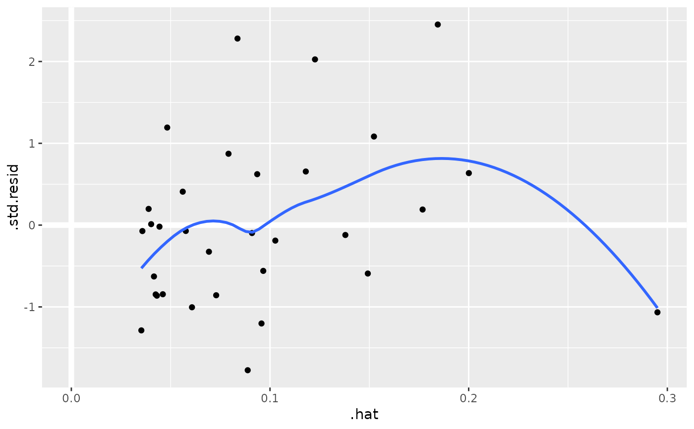
au <- augment(mod, data = mtcars)
ggplot(au, aes(.hat, .std.resid)) +
geom_vline(size = 2, colour = "white", xintercept = 0) +
geom_hline(size = 2, colour = "white", yintercept = 0) +
geom_point() +
geom_smooth(se = FALSE)
#> `geom_smooth()` using method = 'loess' and formula = 'y ~ x'
# predict on new data without outcome variable. Output does not include .resid
newdata <- newdata |>
select(-mpg)
#> Error in select(newdata, -mpg): unused argument (-mpg)
augment(mod, newdata = newdata)
#> # A tibble: 6 × 14
#> .rownames mpg cyl disp hp drat wt qsec vs am gear
#> <chr> <dbl> <dbl> <dbl> <dbl> <dbl> <dbl> <dbl> <dbl> <dbl> <dbl>
#> 1 Mazda RX4 21 6 160 110 3.9 3.62 16.5 0 1 4
#> 2 Mazda RX… 21 6 160 110 3.9 3.88 17.0 0 1 4
#> 3 Datsun 7… 22.8 4 108 93 3.85 3.32 18.6 1 1 4
#> 4 Hornet 4… 21.4 6 258 110 3.08 4.22 19.4 1 0 3
#> 5 Hornet S… 18.7 8 360 175 3.15 4.44 17.0 0 0 3
#> 6 Valiant 18.1 6 225 105 2.76 4.46 20.2 1 0 3
#> # ℹ 3 more variables: carb <dbl>, .fitted <dbl>, .resid <dbl>
au <- augment(mod, data = mtcars)
ggplot(au, aes(.hat, .std.resid)) +
geom_vline(size = 2, colour = "white", xintercept = 0) +
geom_hline(size = 2, colour = "white", yintercept = 0) +
geom_point() +
geom_smooth(se = FALSE)
#> `geom_smooth()` using method = 'loess' and formula = 'y ~ x'
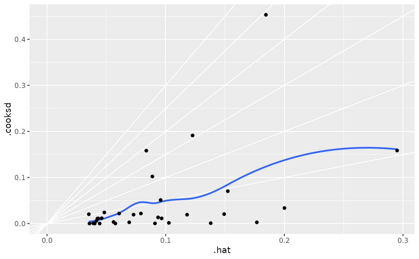
 plot(mod, which = 6)
 ggplot(au, aes(.hat, .cooksd)) +
geom_vline(xintercept = 0, colour = NA) +
geom_abline(slope = seq(0, 3, by = 0.5), colour = "white") +
geom_smooth(se = FALSE) +
geom_point()
#> `geom_smooth()` using method = 'loess' and formula = 'y ~ x'
ggplot(au, aes(.hat, .cooksd)) +
geom_vline(xintercept = 0, colour = NA) +
geom_abline(slope = seq(0, 3, by = 0.5), colour = "white") +
geom_smooth(se = FALSE) +
geom_point()
#> `geom_smooth()` using method = 'loess' and formula = 'y ~ x'
 # column-wise models
a <- matrix(rnorm(20), nrow = 10)
b <- a + rnorm(length(a))
result <- lm(b ~ a)
tidy(result)
#> # A tibble: 6 × 6
#> response term estimate std.error statistic p.value
#> <chr> <chr> <dbl> <dbl> <dbl> <dbl>
#> 1 Y1 (Intercept) -0.276 0.215 -1.28 0.242
#> 2 Y1 a1 0.912 0.273 3.35 0.0123
#> 3 Y1 a2 -0.241 0.195 -1.24 0.256
#> 4 Y2 (Intercept) -0.803 0.448 -1.79 0.116
#> 5 Y2 a1 -0.304 0.566 -0.538 0.607
#> 6 Y2 a2 1.59 0.406 3.93 0.00571
# column-wise models
a <- matrix(rnorm(20), nrow = 10)
b <- a + rnorm(length(a))
result <- lm(b ~ a)
tidy(result)
#> # A tibble: 6 × 6
#> response term estimate std.error statistic p.value
#> <chr> <chr> <dbl> <dbl> <dbl> <dbl>
#> 1 Y1 (Intercept) -0.276 0.215 -1.28 0.242
#> 2 Y1 a1 0.912 0.273 3.35 0.0123
#> 3 Y1 a2 -0.241 0.195 -1.24 0.256
#> 4 Y2 (Intercept) -0.803 0.448 -1.79 0.116
#> 5 Y2 a1 -0.304 0.566 -0.538 0.607
#> 6 Y2 a2 1.59 0.406 3.93 0.00571