Augment data with information from a(n) coxph object

Augment accepts a model object and a dataset and adds information about each observation in the dataset. Most commonly, this includes predicted values in the .fitted column, residuals in the .resid column, and standard errors for the fitted values in a .se.fit column. New columns always begin with a . prefix to avoid overwriting columns in the original dataset.

Users may pass data to augment via either the data argument or the newdata argument. If the user passes data to the data argument, it must be exactly the data that was used to fit the model object. Pass datasets to newdata to augment data that was not used during model fitting. This still requires that at least all predictor variable columns used to fit the model are present. If the original outcome variable used to fit the model is not included in newdata, then no .resid column will be included in the output.

Augment will often behave differently depending on whether data or newdata is given. This is because there is often information associated with training observations (such as influences or related) measures that is not meaningfully defined for new observations.

For convenience, many augment methods provide default data arguments, so that augment(fit) will return the augmented training data. In these cases, augment tries to reconstruct the original data based on the model object with varying degrees of success.

The augmented dataset is always returned as a tibble::tibble with the same number of rows as the passed dataset. This means that the passed data must be coercible to a tibble. If a predictor enters the model as part of a matrix of covariates, such as when the model formula uses splines::ns(), stats::poly(), or survival::Surv(), it is represented as a matrix column.

We are in the process of defining behaviors for models fit with various na.action arguments, but make no guarantees about behavior when data is missing at this time.

Usage

# S3 method for class 'coxph'
augment(
  x,
  data = model.frame(x),
  newdata = NULL,
  type.predict = "lp",
  type.residuals = "martingale",
  ...
)

Arguments

x

A coxph object returned from survival::coxph().

data

A base::data.frame or tibble::tibble() containing the original data that was used to produce the object x. Defaults to stats::model.frame(x) so that augment(my_fit) returns the augmented original data. Do not pass new data to the data argument. Augment will report information such as influence and cooks distance for data passed to the data argument. These measures are only defined for the original training data.

newdata

A base::data.frame() or tibble::tibble() containing all the original predictors used to create x. Defaults to NULL, indicating that nothing has been passed to newdata. If newdata is specified, the data argument will be ignored.

type.predict

Character indicating type of prediction to use. Passed to the type argument of the stats::predict() generic. Allowed arguments vary with model class, so be sure to read the predict.my_class documentation.

type.residuals

Character indicating type of residuals to use. Passed to the type argument of stats::residuals() generic. Allowed arguments vary with model class, so be sure to read the residuals.my_class documentation.

...

Additional arguments. Not used. Needed to match generic signature only. Cautionary note: Misspelled arguments will be absorbed in ..., where they will be ignored. If the misspelled argument has a default value, the default value will be used. For example, if you pass conf.lvel = 0.9, all computation will proceed using conf.level = 0.95. Two exceptions here are:

tidy() methods will warn when supplied an exponentiate argument if it will be ignored.
augment() methods will warn when supplied a newdata argument if it will be ignored.

Details

When the modeling was performed with na.action = "na.omit" (as is the typical default), rows with NA in the initial data are omitted entirely from the augmented data frame. When the modeling was performed with na.action = "na.exclude", one should provide the original data as a second argument, at which point the augmented data will contain those rows (typically with NAs in place of the new columns). If the original data is not provided to augment() and na.action = "na.exclude", a warning is raised and the incomplete rows are dropped.

Value

A tibble::tibble() with columns:

.fitted: Fitted or predicted value.
.resid: The difference between observed and fitted values.
.se.fit: Standard errors of fitted values.

Examples


# load libraries for models and data
library(survival)

# fit model
cfit <- coxph(Surv(time, status) ~ age + sex, lung)

# summarize model fit with tidiers
tidy(cfit)
#> # A tibble: 2 × 5
#>   term  estimate std.error statistic p.value
#>   <chr>    <dbl>     <dbl>     <dbl>   <dbl>
#> 1 age     0.0170   0.00922      1.85 0.0646 
#> 2 sex    -0.513    0.167       -3.06 0.00218
tidy(cfit, exponentiate = TRUE)
#> # A tibble: 2 × 5
#>   term  estimate std.error statistic p.value
#>   <chr>    <dbl>     <dbl>     <dbl>   <dbl>
#> 1 age      1.02    0.00922      1.85 0.0646 
#> 2 sex      0.599   0.167       -3.06 0.00218

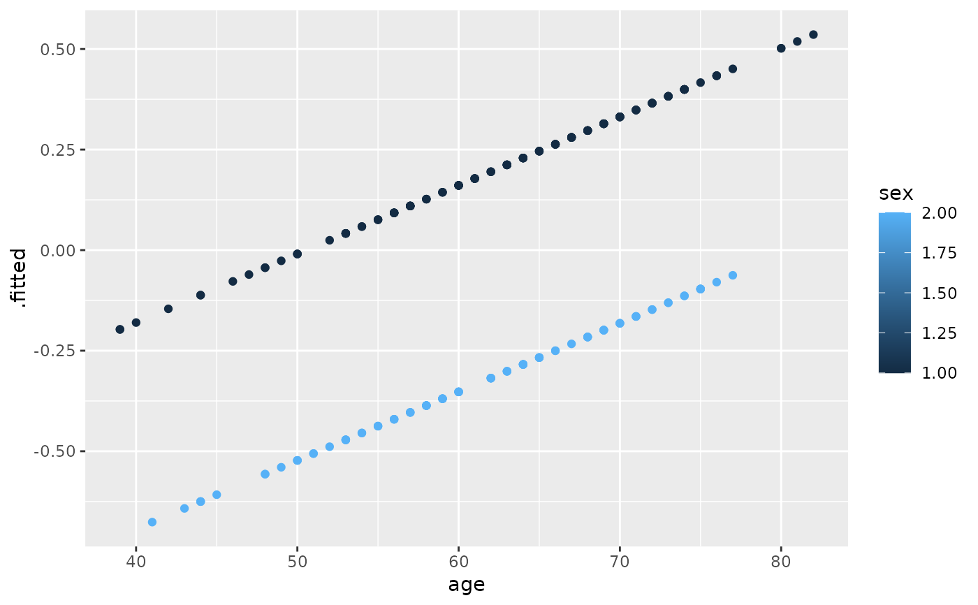
lp <- augment(cfit, lung)
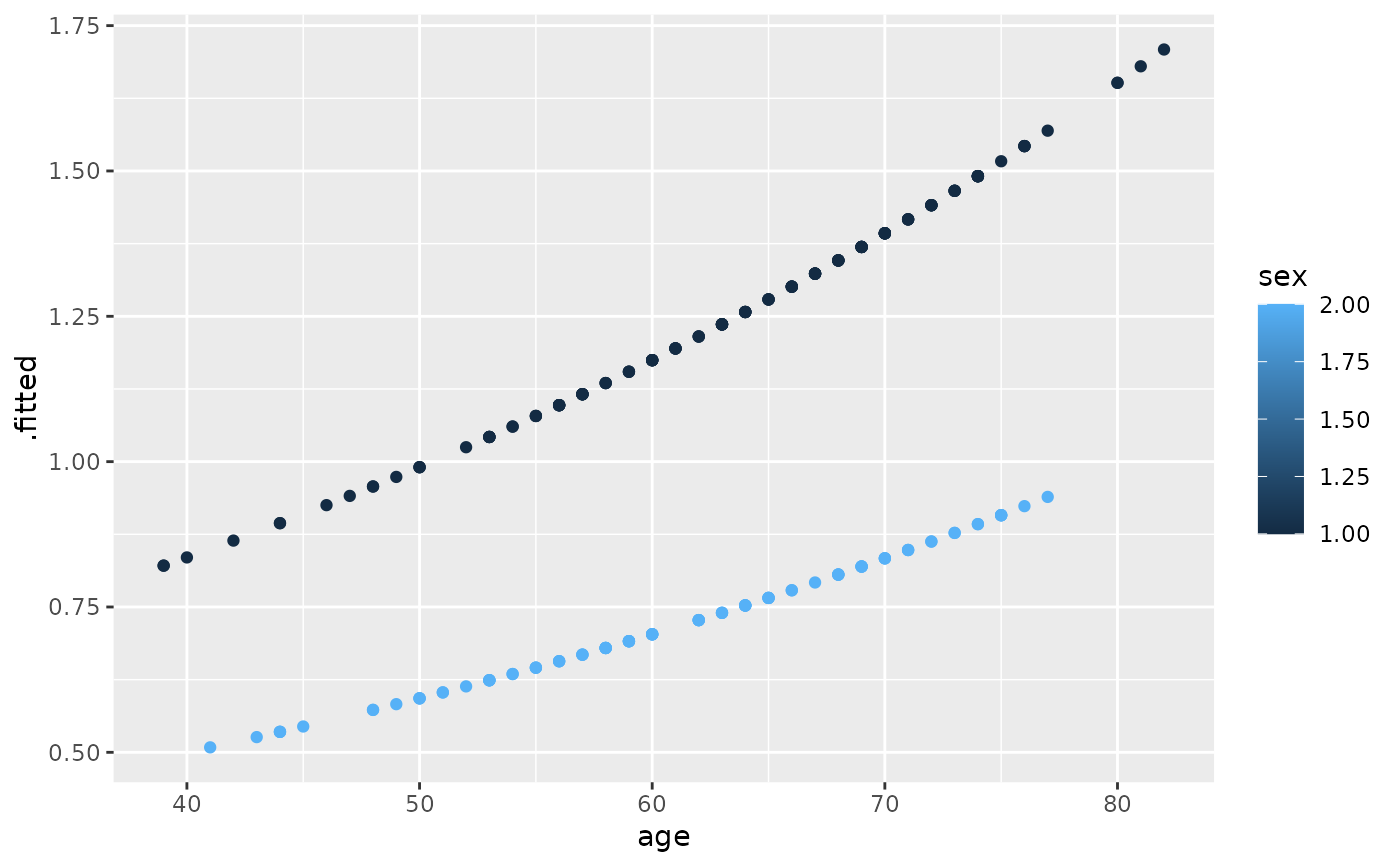
risks <- augment(cfit, lung, type.predict = "risk")
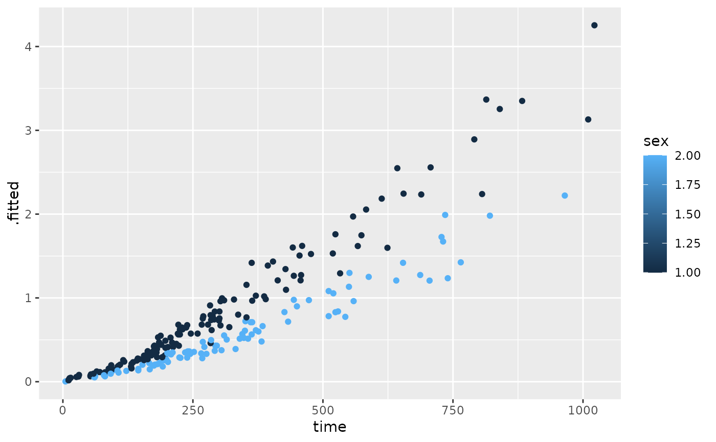
expected <- augment(cfit, lung, type.predict = "expected")

glance(cfit)
#> # A tibble: 1 × 18
#>       n nevent statistic.log p.value.log statistic.sc p.value.sc
#>   <int>  <dbl>         <dbl>       <dbl>        <dbl>      <dbl>
#> 1   228    165          14.1    0.000857         13.7    0.00105
#> # ℹ 12 more variables: statistic.wald <dbl>, p.value.wald <dbl>,
#> #   statistic.robust <dbl>, p.value.robust <dbl>, r.squared <dbl>,
#> #   r.squared.max <dbl>, concordance <dbl>,
#> #   std.error.concordance <dbl>, logLik <dbl>, AIC <dbl>, BIC <dbl>,
#> #   nobs <dbl>

# also works on clogit models
resp <- levels(logan$occupation)
n <- nrow(logan)
indx <- rep(1:n, length(resp))
logan2 <- data.frame(
  logan[indx, ],
  id = indx,
  tocc = factor(rep(resp, each = n))
)

logan2$case <- (logan2$occupation == logan2$tocc)

cl <- clogit(case ~ tocc + tocc:education + strata(id), logan2)

tidy(cl)
#> # A tibble: 9 × 5
#>   term                       estimate std.error statistic   p.value
#>   <chr>                         <dbl>     <dbl>     <dbl>     <dbl>
#> 1 toccfarm                     -1.90     1.38       -1.37  1.70e- 1
#> 2 toccoperatives                1.17     0.566       2.06  3.91e- 2
#> 3 toccprofessional             -8.10     0.699     -11.6   4.45e-31
#> 4 toccsales                    -5.03     0.770      -6.53  6.54e-11
#> 5 tocccraftsmen:education      -0.332    0.0569     -5.84  5.13e- 9
#> 6 toccfarm:education           -0.370    0.116      -3.18  1.47e- 3
#> 7 toccoperatives:education     -0.422    0.0584     -7.23  4.98e-13
#> 8 toccprofessional:education    0.278    0.0510      5.45  4.94e- 8
#> 9 toccsales:education          NA        0          NA    NA       
glance(cl)
#> # A tibble: 1 × 18
#>       n nevent statistic.log p.value.log statistic.sc p.value.sc
#>   <int>  <dbl>         <dbl>       <dbl>        <dbl>      <dbl>
#> 1  4190    838          666.   1.90e-138         682.  5.01e-142
#> # ℹ 12 more variables: statistic.wald <dbl>, p.value.wald <dbl>,
#> #   statistic.robust <dbl>, p.value.robust <dbl>, r.squared <dbl>,
#> #   r.squared.max <dbl>, concordance <dbl>,
#> #   std.error.concordance <dbl>, logLik <dbl>, AIC <dbl>, BIC <dbl>,
#> #   nobs <dbl>

library(ggplot2)

ggplot(lp, aes(age, .fitted, color = sex)) +
  geom_point()


ggplot(risks, aes(age, .fitted, color = sex)) +
  geom_point()


ggplot(expected, aes(time, .fitted, color = sex)) +
  geom_point()