Glance accepts a model object and returns a tibble::tibble()
with exactly one row of model summaries. The summaries are typically
goodness of fit measures, p-values for hypothesis tests on residuals,
or model convergence information.
Glance never returns information from the original call to the modeling function. This includes the name of the modeling function or any arguments passed to the modeling function.
Glance does not calculate summary measures. Rather, it farms out these
computations to appropriate methods and gathers the results together.
Sometimes a goodness of fit measure will be undefined. In these cases
the measure will be reported as NA.
Glance returns the same number of columns regardless of whether the
model matrix is rank-deficient or not. If so, entries in columns
that no longer have a well-defined value are filled in with an NA
of the appropriate type.
Usage
# S3 method for class 'survfit'
glance(x, ...)
Arguments
- x
An
survfitobject returned fromsurvival::survfit().- ...
Additional arguments passed to
survival::summary.survfit(). Important arguments includermean.
See also
Other cch tidiers:
glance.cch(),
tidy.cch()
Other survival tidiers:
augment.coxph(),
augment.survreg(),
glance.aareg(),
glance.cch(),
glance.coxph(),
glance.pyears(),
glance.survdiff(),
glance.survexp(),
glance.survreg(),
tidy.aareg(),
tidy.cch(),
tidy.coxph(),
tidy.pyears(),
tidy.survdiff(),
tidy.survexp(),
tidy.survfit(),
tidy.survreg()
Value
A tibble::tibble() with exactly one row and columns:
- events
Number of events.
- n.max
Maximum number of subjects at risk.
- n.start
Initial number of subjects at risk.
- nobs
Number of observations used.
- records
Number of observations
- rmean
Restricted mean (see [survival::print.survfit()]).
- rmean.std.error
Restricted mean standard error.
- conf.low
lower end of confidence interval on median
- conf.high
upper end of confidence interval on median
- median
median survival
Examples
# load libraries for models and data
library(survival)
# fit model
cfit <- coxph(Surv(time, status) ~ age + sex, lung)
sfit <- survfit(cfit)
# summarize model fit with tidiers + visualization
tidy(sfit)
#> # A tibble: 186 × 8
#> time n.risk n.event n.censor estimate std.error conf.high conf.low
#> <dbl> <dbl> <dbl> <dbl> <dbl> <dbl> <dbl> <dbl>
#> 1 5 228 1 0 0.996 0.00419 1 0.988
#> 2 11 227 3 0 0.983 0.00845 1.000 0.967
#> 3 12 224 1 0 0.979 0.00947 0.997 0.961
#> 4 13 223 2 0 0.971 0.0113 0.992 0.949
#> 5 15 221 1 0 0.966 0.0121 0.990 0.944
#> 6 26 220 1 0 0.962 0.0129 0.987 0.938
#> 7 30 219 1 0 0.958 0.0136 0.984 0.933
#> 8 31 218 1 0 0.954 0.0143 0.981 0.927
#> 9 53 217 2 0 0.945 0.0157 0.975 0.917
#> 10 54 215 1 0 0.941 0.0163 0.972 0.911
#> # ℹ 176 more rows
glance(sfit)
#> # A tibble: 1 × 10
#> records n.max n.start events rmean rmean.std.error median conf.low
#> <dbl> <dbl> <dbl> <dbl> <dbl> <dbl> <dbl> <dbl>
#> 1 228 228 228 165 381. 20.3 320 285
#> # ℹ 2 more variables: conf.high <dbl>, nobs <int>
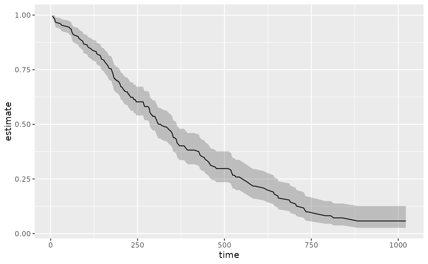
library(ggplot2)
ggplot(tidy(sfit), aes(time, estimate)) +
geom_line() +
geom_ribbon(aes(ymin = conf.low, ymax = conf.high), alpha = .25)
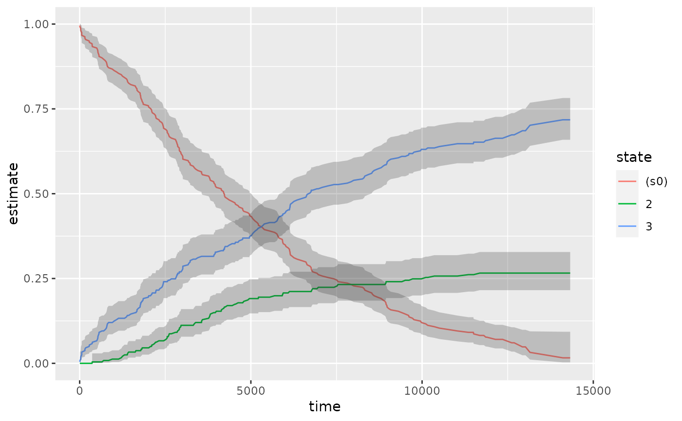
 # multi-state
fitCI <- survfit(Surv(stop, status * as.numeric(event), type = "mstate") ~ 1,
data = mgus1, subset = (start == 0)
)
#> Warning: type= 'mstate' is deprecated, use a factor variable as status
td_multi <- tidy(fitCI)
td_multi
#> # A tibble: 711 × 9
#> time n.risk n.event n.censor estimate std.error conf.high conf.low
#> <dbl> <dbl> <dbl> <dbl> <dbl> <dbl> <dbl> <dbl>
#> 1 6 241 0 0 0.996 0.00414 1 0.988
#> 2 7 240 0 0 0.992 0.00584 1 0.980
#> 3 31 239 0 0 0.988 0.00714 1 0.974
#> 4 32 238 0 0 0.983 0.00823 1.000 0.967
#> 5 39 237 0 0 0.979 0.00918 0.997 0.961
#> 6 60 236 0 0 0.975 0.0100 0.995 0.956
#> 7 61 235 0 0 0.967 0.0115 0.990 0.944
#> 8 152 233 0 0 0.963 0.0122 0.987 0.939
#> 9 153 232 0 0 0.959 0.0128 0.984 0.934
#> 10 174 231 0 0 0.954 0.0134 0.981 0.928
#> # ℹ 701 more rows
#> # ℹ 1 more variable: state <chr>
ggplot(td_multi, aes(time, estimate, group = state)) +
geom_line(aes(color = state)) +
geom_ribbon(aes(ymin = conf.low, ymax = conf.high), alpha = .25)
# multi-state
fitCI <- survfit(Surv(stop, status * as.numeric(event), type = "mstate") ~ 1,
data = mgus1, subset = (start == 0)
)
#> Warning: type= 'mstate' is deprecated, use a factor variable as status
td_multi <- tidy(fitCI)
td_multi
#> # A tibble: 711 × 9
#> time n.risk n.event n.censor estimate std.error conf.high conf.low
#> <dbl> <dbl> <dbl> <dbl> <dbl> <dbl> <dbl> <dbl>
#> 1 6 241 0 0 0.996 0.00414 1 0.988
#> 2 7 240 0 0 0.992 0.00584 1 0.980
#> 3 31 239 0 0 0.988 0.00714 1 0.974
#> 4 32 238 0 0 0.983 0.00823 1.000 0.967
#> 5 39 237 0 0 0.979 0.00918 0.997 0.961
#> 6 60 236 0 0 0.975 0.0100 0.995 0.956
#> 7 61 235 0 0 0.967 0.0115 0.990 0.944
#> 8 152 233 0 0 0.963 0.0122 0.987 0.939
#> 9 153 232 0 0 0.959 0.0128 0.984 0.934
#> 10 174 231 0 0 0.954 0.0134 0.981 0.928
#> # ℹ 701 more rows
#> # ℹ 1 more variable: state <chr>
ggplot(td_multi, aes(time, estimate, group = state)) +
geom_line(aes(color = state)) +
geom_ribbon(aes(ymin = conf.low, ymax = conf.high), alpha = .25)