Tidy summarizes information about the components of a model. A model component might be a single term in a regression, a single hypothesis, a cluster, or a class. Exactly what tidy considers to be a model component varies across models but is usually self-evident. If a model has several distinct types of components, you will need to specify which components to return.
Usage
# S3 method for class 'survreg'
tidy(x, conf.level = 0.95, conf.int = FALSE, ...)
Arguments
- x
An
survregobject returned fromsurvival::survreg().- conf.level
The confidence level to use for the confidence interval if
conf.int = TRUE. Must be strictly greater than 0 and less than 1. Defaults to 0.95, which corresponds to a 95 percent confidence interval.- conf.int
Logical indicating whether or not to include a confidence interval in the tidied output. Defaults to
FALSE.- ...
Additional arguments. Not used. Needed to match generic signature only. Cautionary note: Misspelled arguments will be absorbed in
..., where they will be ignored. If the misspelled argument has a default value, the default value will be used. For example, if you passconf.lvel = 0.9, all computation will proceed usingconf.level = 0.95. Two exceptions here are:
See also
Other survreg tidiers:
augment.survreg(),
glance.survreg()
Other survival tidiers:
augment.coxph(),
augment.survreg(),
glance.aareg(),
glance.cch(),
glance.coxph(),
glance.pyears(),
glance.survdiff(),
glance.survexp(),
glance.survfit(),
glance.survreg(),
tidy.aareg(),
tidy.cch(),
tidy.coxph(),
tidy.pyears(),
tidy.survdiff(),
tidy.survexp(),
tidy.survfit()
Value
A tibble::tibble() with columns:
- conf.high
Upper bound on the confidence interval for the estimate.
- conf.low
Lower bound on the confidence interval for the estimate.
- estimate
The estimated value of the regression term.
- p.value
The two-sided p-value associated with the observed statistic.
- statistic
The value of a T-statistic to use in a hypothesis that the regression term is non-zero.
- std.error
The standard error of the regression term.
- term
The name of the regression term.
Examples
# load libraries for models and data
library(survival)
# fit model
sr <- survreg(
Surv(futime, fustat) ~ ecog.ps + rx,
ovarian,
dist = "exponential"
)
# summarize model fit with tidiers + visualization
tidy(sr)
#> # A tibble: 3 × 5
#> term estimate std.error statistic p.value
#> <chr> <dbl> <dbl> <dbl> <dbl>
#> 1 (Intercept) 6.96 1.32 5.27 0.000000139
#> 2 ecog.ps -0.433 0.587 -0.738 0.461
#> 3 rx 0.582 0.587 0.991 0.322
augment(sr, ovarian)
#> # A tibble: 26 × 9
#> futime fustat age resid.ds rx ecog.ps .fitted .se.fit .resid
#> <dbl> <dbl> <dbl> <dbl> <dbl> <dbl> <dbl> <dbl> <dbl>
#> 1 59 1 72.3 2 1 1 1224. 639. -1165.
#> 2 115 1 74.5 2 1 1 1224. 639. -1109.
#> 3 156 1 66.5 2 1 2 794. 350. -638.
#> 4 421 0 53.4 2 2 1 2190. 1202. -1769.
#> 5 431 1 50.3 2 1 1 1224. 639. -793.
#> 6 448 0 56.4 1 1 2 794. 350. -346.
#> 7 464 1 56.9 2 2 2 1420. 741. -956.
#> 8 475 1 59.9 2 2 2 1420. 741. -945.
#> 9 477 0 64.2 2 1 1 1224. 639. -747.
#> 10 563 1 55.2 1 2 2 1420. 741. -857.
#> # ℹ 16 more rows
glance(sr)
#> # A tibble: 1 × 9
#> iter df statistic logLik AIC BIC df.residual nobs p.value
#> <int> <int> <dbl> <dbl> <dbl> <dbl> <int> <int> <dbl>
#> 1 4 3 1.67 -97.2 200. 204. 23 26 0.434
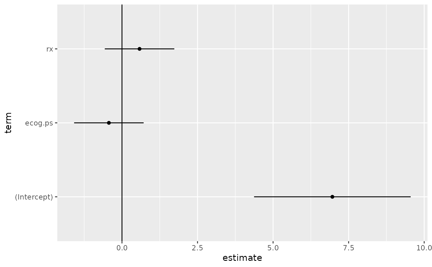
# coefficient plot
td <- tidy(sr, conf.int = TRUE)
library(ggplot2)
ggplot(td, aes(estimate, term)) +
geom_point() +
geom_errorbarh(aes(xmin = conf.low, xmax = conf.high), height = 0) +
geom_vline(xintercept = 0)
#> `height` was translated to `width`.