Glance at a(n) coxph object

Glance accepts a model object and returns a tibble::tibble() with exactly one row of model summaries. The summaries are typically goodness of fit measures, p-values for hypothesis tests on residuals, or model convergence information.

Glance never returns information from the original call to the modeling function. This includes the name of the modeling function or any arguments passed to the modeling function.

Glance does not calculate summary measures. Rather, it farms out these computations to appropriate methods and gathers the results together. Sometimes a goodness of fit measure will be undefined. In these cases the measure will be reported as NA.

Glance returns the same number of columns regardless of whether the model matrix is rank-deficient or not. If so, entries in columns that no longer have a well-defined value are filled in with an NA of the appropriate type.

Usage

# S3 method for class 'coxph'
glance(x, ...)

Arguments

x

A coxph object returned from survival::coxph().

...

For tidy(), additional arguments passed to summary(x, ...). Otherwise ignored.

See also

glance(), survival::coxph()

Other coxph tidiers: augment.coxph(), tidy.coxph()

Other survival tidiers: augment.coxph(), augment.survreg(), glance.aareg(), glance.cch(), glance.pyears(), glance.survdiff(), glance.survexp(), glance.survfit(), glance.survreg(), tidy.aareg(), tidy.cch(), tidy.coxph(), tidy.pyears(), tidy.survdiff(), tidy.survexp(), tidy.survfit(), tidy.survreg()

Value

A tibble::tibble() with exactly one row and columns:

AIC

Akaike's Information Criterion for the model.

BIC

Bayesian Information Criterion for the model.

logLik

The log-likelihood of the model. [stats::logLik()] may be a useful reference.

n

The total number of observations.

nevent

Number of events.

nobs

Number of observations used.

See survival::coxph.object for additional column descriptions.

Examples

# load libraries for models and data
library(survival)

# fit model
cfit <- coxph(Surv(time, status) ~ age + sex, lung)

# summarize model fit with tidiers
tidy(cfit)
#> # A tibble: 2 × 5
#>   term  estimate std.error statistic p.value
#>   <chr>    <dbl>     <dbl>     <dbl>   <dbl>
#> 1 age     0.0170   0.00922      1.85 0.0646 
#> 2 sex    -0.513    0.167       -3.06 0.00218
tidy(cfit, exponentiate = TRUE)
#> # A tibble: 2 × 5
#>   term  estimate std.error statistic p.value
#>   <chr>    <dbl>     <dbl>     <dbl>   <dbl>
#> 1 age      1.02    0.00922      1.85 0.0646 
#> 2 sex      0.599   0.167       -3.06 0.00218

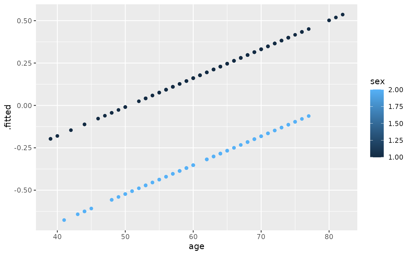
lp <- augment(cfit, lung)
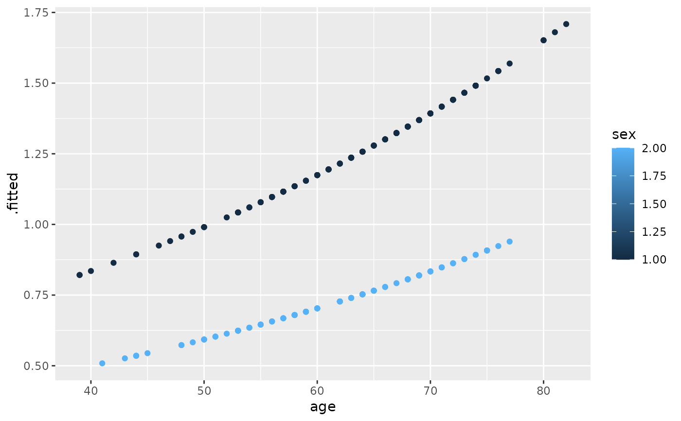
risks <- augment(cfit, lung, type.predict = "risk")
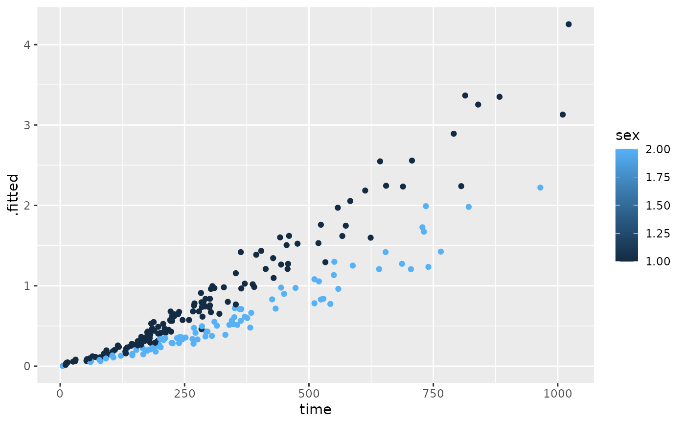
expected <- augment(cfit, lung, type.predict = "expected")

glance(cfit)
#> # A tibble: 1 × 18
#>       n nevent statistic.log p.value.log statistic.sc p.value.sc
#>   <int>  <dbl>         <dbl>       <dbl>        <dbl>      <dbl>
#> 1   228    165          14.1    0.000857         13.7    0.00105
#> # ℹ 12 more variables: statistic.wald <dbl>, p.value.wald <dbl>,
#> #   statistic.robust <dbl>, p.value.robust <dbl>, r.squared <dbl>,
#> #   r.squared.max <dbl>, concordance <dbl>, std.error.concordance <dbl>,
#> #   logLik <dbl>, AIC <dbl>, BIC <dbl>, nobs <dbl>

# also works on clogit models
resp <- levels(logan$occupation)
n <- nrow(logan)
indx <- rep(1:n, length(resp))
logan2 <- data.frame(
  logan[indx, ],
  id = indx,
  tocc = factor(rep(resp, each = n))
)

logan2$case <- (logan2$occupation == logan2$tocc)

cl <- clogit(case ~ tocc + tocc:education + strata(id), logan2)

tidy(cl)
#> # A tibble: 9 × 5
#>   term                       estimate std.error statistic   p.value
#>   <chr>                         <dbl>     <dbl>     <dbl>     <dbl>
#> 1 toccfarm                     -1.90     1.38       -1.37  1.70e- 1
#> 2 toccoperatives                1.17     0.566       2.06  3.91e- 2
#> 3 toccprofessional             -8.10     0.699     -11.6   4.45e-31
#> 4 toccsales                    -5.03     0.770      -6.53  6.54e-11
#> 5 tocccraftsmen:education      -0.332    0.0569     -5.84  5.13e- 9
#> 6 toccfarm:education           -0.370    0.116      -3.18  1.47e- 3
#> 7 toccoperatives:education     -0.422    0.0584     -7.23  4.98e-13
#> 8 toccprofessional:education    0.278    0.0510      5.45  4.94e- 8
#> 9 toccsales:education          NA        0          NA    NA       
glance(cl)
#> # A tibble: 1 × 18
#>       n nevent statistic.log p.value.log statistic.sc p.value.sc
#>   <int>  <dbl>         <dbl>       <dbl>        <dbl>      <dbl>
#> 1  4190    838          666.   1.90e-138         682.  5.01e-142
#> # ℹ 12 more variables: statistic.wald <dbl>, p.value.wald <dbl>,
#> #   statistic.robust <dbl>, p.value.robust <dbl>, r.squared <dbl>,
#> #   r.squared.max <dbl>, concordance <dbl>, std.error.concordance <dbl>,
#> #   logLik <dbl>, AIC <dbl>, BIC <dbl>, nobs <dbl>

library(ggplot2)

ggplot(lp, aes(age, .fitted, color = sex)) +
  geom_point()


ggplot(risks, aes(age, .fitted, color = sex)) +
  geom_point()


ggplot(expected, aes(time, .fitted, color = sex)) +
  geom_point()