Glance at a(n) cch object

Glance accepts a model object and returns a tibble::tibble() with exactly one row of model summaries. The summaries are typically goodness of fit measures, p-values for hypothesis tests on residuals, or model convergence information.

Glance never returns information from the original call to the modeling function. This includes the name of the modeling function or any arguments passed to the modeling function.

Glance does not calculate summary measures. Rather, it farms out these computations to appropriate methods and gathers the results together. Sometimes a goodness of fit measure will be undefined. In these cases the measure will be reported as NA.

Glance returns the same number of columns regardless of whether the model matrix is rank-deficient or not. If so, entries in columns that no longer have a well-defined value are filled in with an NA of the appropriate type.

Usage

# S3 method for class 'cch'
glance(x, ...)

Arguments

x

An cch object returned from survival::cch().

...

Additional arguments. Not used. Needed to match generic signature only. Cautionary note: Misspelled arguments will be absorbed in ..., where they will be ignored. If the misspelled argument has a default value, the default value will be used. For example, if you pass conf.lvel = 0.9, all computation will proceed using conf.level = 0.95. Two exceptions here are:

• tidy() methods will warn when supplied an exponentiate argument if it will be ignored.

• augment() methods will warn when supplied a newdata argument if it will be ignored.

See also

glance(), survival::cch()

Other cch tidiers: glance.survfit(), tidy.cch()

Other survival tidiers: augment.coxph(), augment.survreg(), glance.aareg(), glance.coxph(), glance.pyears(), glance.survdiff(), glance.survexp(), glance.survfit(), glance.survreg(), tidy.aareg(), tidy.cch(), tidy.coxph(), tidy.pyears(), tidy.survdiff(), tidy.survexp(), tidy.survfit(), tidy.survreg()

Value

A tibble::tibble() with exactly one row and columns:

iter

Iterations of algorithm/fitting procedure completed.

p.value

P-value corresponding to the test statistic.

rscore

Robust log-rank statistic

score

Score.

n

number of predictions

nevent

number of events

Examples

# load libraries for models and data
library(survival)

# examples come from cch documentation
subcoh <- nwtco$in.subcohort
selccoh <- with(nwtco, rel == 1 | subcoh == 1)
ccoh.data <- nwtco[selccoh, ]
ccoh.data$subcohort <- subcoh[selccoh]

# central-lab histology
ccoh.data$histol <- factor(ccoh.data$histol, labels = c("FH", "UH"))

# tumour stage
ccoh.data$stage <- factor(ccoh.data$stage, labels = c("I", "II", "III", "IV"))
ccoh.data$age <- ccoh.data$age / 12 # age in years

# fit model
fit.ccP <- cch(Surv(edrel, rel) ~ stage + histol + age,
  data = ccoh.data,
  subcoh = ~subcohort, id = ~seqno, cohort.size = 4028
)

# summarize model fit with tidiers + visualization
tidy(fit.ccP)
#> # A tibble: 5 × 7
#>   term     estimate std.error statistic  p.value conf.low conf.high
#>   <chr>       <dbl>     <dbl>     <dbl>    <dbl>    <dbl>     <dbl>
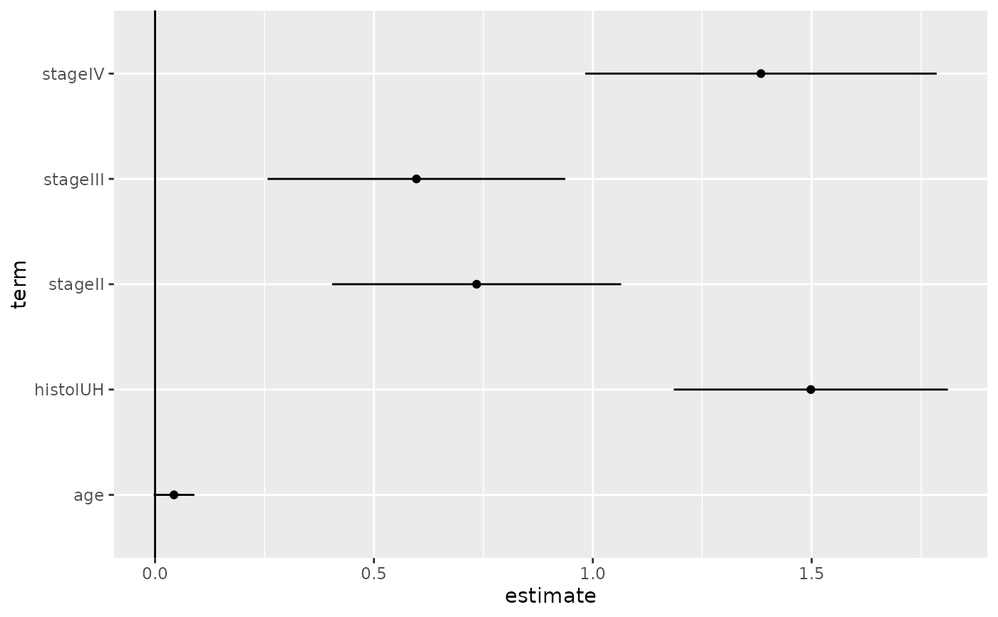
#> 1 stageII    0.735     0.168       4.36 1.30e- 5  0.404      1.06  
#> 2 stageIII   0.597     0.173       3.44 5.77e- 4  0.257      0.937 
#> 3 stageIV    1.38      0.205       6.76 1.40e-11  0.983      1.79  
#> 4 histolUH   1.50      0.160       9.38 0         1.19       1.81  
#> 5 age        0.0433    0.0237      1.82 6.83e- 2 -0.00324    0.0898

# coefficient plot
library(ggplot2)

ggplot(tidy(fit.ccP), aes(x = estimate, y = term)) +
  geom_point() +
  geom_errorbarh(aes(xmin = conf.low, xmax = conf.high), height = 0) +
  geom_vline(xintercept = 0)